Evaluating Value at Risk Methodologies: Accuracy versus Computational Time

Transcription

1 Financial Institutions Center Evaluating Value at Risk Methodologies: Accuracy versus Computational Time by Matthew Pritsker 96-48

2 THE WHARTON FINANCIAL INSTITUTIONS CENTER The Wharton Financial Institutions Center provides a multi-disciplinary research approach to the problems and opportunities facing the financial services industry in its search for competitive excellence. The Center's research focuses on the issues related to managing risk at the firm level as well as ways to improve productivity and performance. The Center fosters the development of a community of faculty, visiting scholars and Ph.D. candidates whose research interests complement and support the mission of the Center. The Center works closely with industry executives and practitioners to ensure that its research is informed by the operating realities and competitive demands facing industry participants as they pursue competitive excellence. Copies of the working papers summarized here are available from the Center. If you would like to learn more about the Center or become a member of our research community, please let us know of your interest. Anthony M. Santomero Director The Working Paper Series is made possible by a generous grant from the Alfred P. Sloan Foundation

3 Evaluating Value at Risk Methodologies: Accuracy versus Computational Time 1 First Version: September 1995 Current Version: November 1996 Abstract: Recent research has shown that different methods of computing Value at Risk (VAR) generate widely varying results, suggesting the choice of VAR method is very important. This paper examines six VAR methods, and compares their computational time requirements and their accuracy when the sole source of inaccuracy is errors in approximating nonlinearity. Simulations using portfolios of foreign exchange options showed fairly wide variation in accuracy and unsurprisingly wide variation in computational time. When the computational time and accuracy of the methods were examined together, four methods were superior to the others. The paper also presents a new method for using order statistics to create confidence intervals for the errors and errors as a percent of true value at risk for each VAR method. This makes it possible to easily interpret the implications of VAR errors for the size of shortfalls or surpluses in a firm's risk based capital. Matthew Pritsker is at the Board of Governors of the Federal Reserve System. The views expressed in this paper reflect those of the author and not those of the Board of Governors of the Federal Reserve System or other members of its staff. The author thanks Ruth Wu for extraordinary research assistance, and thanks Jim O'Brien and Phillipe Jorion for extensive comments on an earlier version, and also thanks Vijay Bhasin, Paul Kupiec, Pat White, and Chunsheng Zhou for useful comments and conversations. All errors are the responsibility of the author. Address correspondence to Matt Pritsker, The Federal Reserve Board, Mail Stop 91, Washington, DC 20551, or send to mpritsker@frb.gov. The author's phone number is (202) This paper was presented at the Wharton Financial Institutions Center's conference on Risk Management in Banking, October 13-15, 1996.

4 I Introduction. New methods of measuring and managing risk have evolved in parallel with the growth of the OTC derivatives market. One of these risk measures, known as Value at risk (VAR) has become especially prominent, and now serves as the basis for the most recent BIS market risk based capital requirement. Value at risk is usually defined as the largest loss in portfolio value that would be expected to occur due to changes in market prices over a given period of time in all but a small percentage of circumstances. 1 This percentage is referred to as the confidence level for the value at risk measure. 2 An alternative characterization of value at risk is the amount of capital the firm would require to absorb its portfolio losses in all but a small percentage of circumstances. 3 Value at risk s prominence has grown because of its conceptual simplicity and flexibility. It can be used to measure the risk of an individual instrument, or the risk of an entire portfolio. Value at risk measures are also potentially useful for the short- term management of the firm s risk. For example, if VAR figures are available on a timely basis, then a firm can increase its risk if VAR is too low, or decrease its risk if VAR is too high. While VAR is conceptually simple, and flexible, for VAR figures to be useful, they also need to be reasonably accurate, and they need to be available on a timely enough basis that they can be used for risk management. This will typically involve a tradeoff since the 1 A bibliography of VAR literature that is periodically updated is maintained on the internet by Barry Schacter of the Office of the Comptroller of the Currency and is located at 2 If a firm is expected to lose no more than $10 million over the next day except in l% of circumstances, then its value at risk for a 1 day horizon at a l% confidence level is $10 million. 3 Boudoukh, Richardson, and Whitelaw (1995) propose a different measure of capital adequacy. They suggest measuring risk as the expected largest loss experienced over a fixed period of time. For example, the expected largest daily loss over a period of 20 days. 1

5 most accurate methods may take unacceptably long amounts of time to compute while the methods that take the least time are often the least accurate. The purpose of this paper is to examine the tradeoffs between methods of computing VAR, and to accuracy and computational time among six different highlight the strengths and weaknesses of the various methods. The need to examine accuracy is especially poignant since the most recent Basle market risk capital proposal sets capital requirements based on VAR estimates from a firms' own internal VAR models. In addition it is important to examine accuracy since recent evidence on the accuracy of VAR methods has not been encouraging; different methods of computing VAR tend to generate widely varying results, suggesting that the choice of VAR method is very important. The differences in the results appear to be due to the use of procedures that implicitly use different methods to impute the joint distribution of the factor shocks [Hendricks(1996), Beder (1995)], 4 and due to differences in the treatment of instruments whose payoffs are nonlinear functions of the factors [Marshall and Siegel (1996)]. 5 Tradeoffs between accuracy and computational time are most acute when portfolios contain large holdings of instruments whose payoffs are nonlinear in the underlying risk factors because VAR is the most difficult to compute for these portfolios. However, while the dis- 4 Hendricks(1996) examined 12 different estimates of VAR and found that the standard deviation of their dispersion around the mean of the estimates is between 10 and 15%, indicating that it would not be uncommon for the VAR estimates he considered to differ by 30 to 50% on a daily basis. Beder (1995) examined 8 approaches to computing VAR and found that the low and high estimates of VAR for a given portfolio differed by a factor that ranged from 6 to Marshall and Siegel asked a large number of VAR software vendors to estimate VAR for several portfolios. The distributional assumptions used in the estimations was presumably the same since all of the vendors used a common set of correlations and standard deviations provided by Riskmetrics. Despite common distributional assumptions, VAR estimates varied especially widely for nonlinear instruments suggesting that differences in the treatment of nonlinearities drive the differences in VAR estimates. For portfolios of foreign exchange options, which we will consider later, Marshall and Siegel found that the ratio of standard deviation of VAR estimate to median VAR estimate was 25%. 2

6 persion of VAR estimates for nonlinear portfolios has been documented, there has been relatively little publicly available research that compares the accuracy of the various methods. Moreover, the results that have been reported are often portfolio specific and often reported only in dollar terms. This makes it difficult to make comparisons of results across the VAR literature; it also makes it difficult to relate the results on accuracy to the capital charges under the BIS market-risk based capital proposal. While there has been little publicly available information on the accuracy of the methods, there has been even less reported on the computational feasibility of the various methods. Distinguishing features of this paper are its focus on accuracy versus computation time for portfolios that exclusively contain nonlinear instruments. An additional important contribution of this paper is that it provides a statistically rigorous and easily interpretable method for gauging the accuracy of the VAR estimates in both dollar terms, and as a percent of true VAR even though true VAR is not known. Before proceeding, it is useful to summarize our empirical results. We examined accuracy and computational time in detail using simulations on test portfolios of foreign exchange options. The results on accuracy varied widely. One method (delta-gamma-minimization) produced results which consistently overstated VAR by very substantial amounts. The results on accuracy for the other methods can be roughly split into two groups, the accuracy of simple methods (delta, and delta-gamma-delta), and the accuracy of relatively complex methods (delta-gamma monte-carlo, modified grid monte-carlo, and monte-carlo with full repricing). The simple methods were generally less accurate than the complex methods and the differences in the performance of the methods were substantial. The results on computational time favored the simple methods, which is not surprising. However, one of the 3

7 complex methods (delta-gamma monte-carlo), also takes a relatively short time to compute, and produces among the most accurate results. Based on the tradeoffs between accuracy and computational time, that method appears to perform the best for the portfolios considered here. However, even for this method, we were able to statistically detect a tendency to overstate or understate true VAR for about 25% of the 500 randomly chosen portfolios from simulation exercise 2. When VAR was over- or underof the average magnitude of the error was about 10% of true stated, a conservative estimate VAR with a standard deviation of about the same amount. In addition from simulation 1, we found that all VAR methods except for monte-carlo with full repricing generated large errors as a percent of VAR for deep out of the money options with a short time to expiration. Although VAR for these options is typically very small, if portfolios contain a large concentration of these options, then the best way to capture the risk of these options may be to use monte-carlo with full repricing. 6 The paper proceeds in six parts. Part II formally overview of various methodologies for its computation. defines value at risk and provides an Part III discusses how to measure the accuracy of VAR computations. Part IV discusses computational time requirements. Part V presents results from our simulations for portfolios of FX options. Part VI concludes. II Methods for Measuring Value at Risk. It is useful to begin our analysis of value at risk with its formal definition. Throughout, we will follow current practice and measure value at risk over a fixed span of time (normalized to one period) in which positions are assumed to remain fixed. Many firms set this span of time to be one day. This amount of time is long enough for risk over this horizon to be worth 6 It is possible to combine monte-carlo methods so that VAR with full repricing is applied to some sets of instruments, while other monte-carlo techniques are applied to other options. 4

8 measuring, and it is short enough that the fixed position may reasonably approximate the firm s one-day or overnight position for risk management purposes. To formally define value at risk requires some notation. Denote V(P t, X t, t) as the value P t, X t, t) as the change in portfolio value between period t and t+l. The cumulative density as: Value at risk for confidence level u is defined in terms of the inverse cumulative density In words, value at risk at confidence level u is the largest loss that is expected to occur except for a set of circumstances with probability u. 7 This is equivalent to defining value and a random component and then define VAR at confidence level u as the u th quantile of the random component. I find this treatment to be less appealing than the approach here because from a risk management and regulatory perspective, VAR should measure a firm s capital adequacy, which is based on its ability to cover both the random and deterministic components of changes in V. An additional reason to prefer my approach is that the deterministic component is itself measured with error since it typically is derived using a first order Taylor series expansion in time to maturity.

9 given I t. The definition of VAR highlights its dependence on the function G 1 which is a conditional function of the instruments X t and the information set I t. 8 Value at Risk methods attempt to implicitly or explicitly make inferences about G 1 (u, I t, X t ) in a neighborhood near confidence level u. In a large portfolio G 1 depends on the joint distribution of potentially tens of thousands of different instruments. This makes it necessary to make simplifying assumptions in order to compute VAR; these assumptions usually take three forms. First, the dimension of the problem is reduced by assuming that the price of the instruments depend on a vector of factors ƒ that are the primary determinants of changes in portfolio value. 9 culated explicitly. Finally, convenient functional forms are often assumed for the distribution Each of these simplifying assumptions is likely to introduce errors in the VAR estimates. The first assumption induces errors if an incorrect or incomplete set of factors is chosen; the second assumption introduces approximation error; and the third assumption introduces error while the errors of the second type are approximation error. Because model error can take so many forms, we choose to abstract from it here by assuming that the factors have been chosen correctly, and the distribution of the factor innovations is correct. This allows 8 All of the information on the risk of the portfolio is contained in the function G(.); a single VAR estimate uses only some of this information. However, as much of the function G(.) as is desired can be recovered using VAR methods by computing VAR for whatever quantiles are desired. The accuracy of the methods will vary based on the quantile. 9 Changes in the value of an instrument are caused by changes in the factors and by instrument-specific idiosyncratic changes. In well-diversified portfolios, only changes in the value of the factors should matter since idiosyncratic changes will be diversified away. If a portfolio is not well diversified, these idiosyncratic factors need to be treated as factors. 6

10 us to focus on the errors induced by the approximations used in each VAR method, and to get a clean measure of these errors. In future work, I hope to incorporate model error in the analysis and examine whether some methods of computing VAR are robust to certain classes of model errors. The different methods of computing VAR are distinguished by their simplifying assumptions. The value at risk methodologies that I consider fall into two broad categories. The first are delta and delta-gamma methods. These methods typically make assumptions that lead to analytic or near analytic tractability for the value at risk computation. The second set of methods use monte-carlo simulation to compute value at risk. Their advantage is they are capable of producing very accurate estimates of value- at-risk, however, these methods are not analytically tractable, and they are very time and computer intensive. Delta and Delta-Gamma methods. The delta and delta-gamma methods typically make the distributional assumption that changes in the factors are distributed normally conditional on today s information: The delta and delta-gamma methods principally differ in their approximation of change in portfolio value. The delta method approximates the change in portfolio value using a first order Taylor series expansion in the factor shocks and the time horizon over which VAR is computed 10 : which VAR is computed. In our case this horizon has been normalized to one time period. Therefore, the 7

11 Delta-gamma methods approximate changes in portfolio value using a Taylor series expansion that is second order in the factor shocks and first order in the VAR time horizon: At this juncture it is important to emphasize that the Taylor expansions and distributional assumptions depend on the choice of factors. This choice can have an important impact on the ability of the Taylor expansions to approximate non-linearity 11, and may also have an important impact on the adequacy of the distributional assumptions. For a given choice of the factors, the first-order approximation and distributional assump- 11 To illustrate the impact of factor choice on a first order Taylor series ability to capture non-linearity, consider a three year bond with annual coupon c and principal 1$. Its price today is where the p(i) are the respective prices of zero coupon bonds expiring i years from today. If the factors are the zero coupon bond prices, then the bond price is clearly a linear function of the factors, requiring at most a first order Taylor series. If instead the factors are the one, two and three year zero coupon interest rates and The example shows that the second set of factors requires a Taylor series of at least order 2 to capture the non-linearity of changes in portfolio value. 12 Allen (1994) refers to the delta method as the correlation method; Wilson (1994) refers to this method as the delta-normal method. 8

12 VAR using this method only requires calculating the inverse cumulative density function of the normal distribution. In this case, elementary calculation shows value at risk at confiof the normal distribution. The delta method s main virtue is its simplicity. This allows value at risk to be computed very rapidly. However, its linear Taylor series approximation may be inappropriate for portfolios whose value is a non-linear function of the factors. The normality assumption is also suspect since many financial time series are fat tailed. 13 The delta-gamma approaches attempt to improve on the delta method by using a second-order Taylor series to capture the nonlinearities of changes in portfolio value. Some of the delta-gamma methods also allow for more flexible assumptions on the distribution of the factor innovations. Delta-gamma methods represent some improvement over the delta method by offering a more flexible functional form for capturing nonlinearity. 14 However, a second order approximation is still not capable of capturing all of the non-linearities of changes in portfolio value. 15 In addition, the nonlinearities that are captured come at the cost of reduced analytic tractability relative to the delta method. The reason is that changes in portfolio using the second order Taylor series expansion are not approximately normally distributed even if the factor innovations are. 16 This loss of normality makes it more difficult to compute 14 Anecdotal evidence suggests that many practitioners using delta-gamma methods set off-diagonal ele- 15 Estrella(1995) highlights the need for caution in applying Taylor expansions by showing that a Taylor series expansion of the Black-Scholes pricing formula in terms of the underlying stock price diverges over some range of prices. However, a Taylor series expanded in log(stock price) does not diverge. 16 Changes in portfolio value in the delta method are approximated using linear combinations of normally distributed random variables. These are distributed normally. The delta-gamma method approximates changes in portfolio value using the sum of linear combinations of normally distributed random variables and second order quadratic terms. Because the quadratic terms have a chi-square distribution, the normality is lost.

13 the G 1 function than in the delta method. Two basic fixes are used to try to finesse this difficulty. The first abandons analytic tractability and approximates G 1 using monte-carlo methods; by contrast, the second attempts to maintain analytic or near-analytic tractability by employing additional distributional assumptions. Many of the papers that use a delta-gamma method for computing VAR refer to the method they use as the delta-gamma method. This nomenclature is inadequate here since I examine the performance of three delta-gamma methods in detail, as well as discussing two recent additions to these methods. Instead, I have chosen names that are somewhat descriptive of how these methods are implemented. The first approach is the delta-gamma monte-carlo method. 17 Under this approach, sponding to the u th percentile of the empirical distribution is the estimate of value at risk. If the second order Taylor approximation is exact, then this estimator will converge to true value at risk as the number of monte-carlo draws approaches infinity. The next approach is the delta-gamma-delta method. I chose to give it this name because it is a delta-gamma based method that maintains most of the simplicity of the l7 This approach is one of those used in Jordan and Mackay (1995). They make their monte-carlo draws using a historical simulation or bootstrap approach. 18 This distribution need not be normal. 10

14 second order Taylor series expansion. 19 For example, if V is a function of one factor, then is: The mean and covariance matrix in the above expressions are but the assumption of normality cannot possibly be correct 20, and should instead be viewed as a convenient assumption that simplifies the computation of VAR. Under this distributional G 1 and hence VAR is simple to calculate in the delta-gamma-delta approach. In this for a large number of factors proceeds along similar lines. 22 The next delta-gamma approach is the delta-gamma-minimization method. 23 It lio value are well approximated quadratically. the greatest loss in portfolio value subject to mathematical terms, this value at risk estimate is the solution to the minimization problem: Technical Document, Third Edition, page 137. that only 2N factors are required to compute value at risk. Details on this transformation are contained in appendix C. 23 This approach is discussed in Wilson (1994). 11

15 where c*(1 u, k) is the u% critical value of the central chi-squared distribution with k degrees of freedom; i.e. l-u% of the probability mass of the central chi-squared distribution with k degrees of freedom is below c* (1 u, k). This approach makes a very strong but not obvious distributional assumption to identify value-at-risk. The distributional assumption is that the value of the portfolio outside of the constraint set is lower than anywhere within the constraint set. If this assumption is correct, and the quadratic approximation for changes in portfolio value is exact, then the value at risk estimate would exactly correspond to the u th quantile of the change in portfolio value. Unfortunately there is little reason to believe that this key distributional assumption will be satisfied and it is realistic to believe that this condition will be violated for a substantial (i.e. non-zero) proportion of the shocks that lie outside the constraint set. 24 This means that typically less than u% of the realizations are below the estimated value-at-risk, and thus the delta-gamma minimization method is very likely to overstate true value at risk. In for a factor shock that lies within the 95% constraint set. In this case, estimated value-atrisk would be minus infinity at the 5% confidence level while true value at risk would be This example is extreme, but illustrates the point that this method is capable of 24 Here is one simple example where the assumption is violated. Suppose a firm has a long equity position. Then if one vector of factor shocks that lies outside the constraint set involves a large loss in the equity market, generating a large loss for the firm, then the opposite of this vector lies outside the constraint set too, but is likely to generate large increase in the value of the firms portfolio. A positive proportion of the factor shocks outside the constraint set are near the one in the example, and will also have the same property. 12

16 generating large errors. It is more likely that at low levels of confidence, as the amount of probability mass outside the constraint set goes to zero, the estimate of value at risk using this method remains conservative but converges to true value at risk (conditional on the second order approximation being exact). This suggests the delta-gamma-minimization method will produce better (i.e. less conservative) estimates of value at risk when the confidence level u is small. The advantage of the delta-gamma-minimization approach is that it does not rely on the incorrect joint normality assumption that is used in the delta-gamma-delta method, and does not require the large number of monte-carlo draws required in the delta-gamma monte-carlo approach. Whether these advantages offset the errors induced by this approach s conservatism is an empirical question. In the sections that follow I will examine the accuracy and computational time requirements of the delta-gamma monte-carlo, delta-gamma-delta, and delta-gamma-minimization methods. For completeness I mention here two additional delta-gamma methods. The first of these was recently introduced by Peter Zangari of J.P. Morgan (1996) and parameterizes a known distribution function so that its first four moments match the first four moments of the delta-gamma approximation to changes in portfolio value. The cumulative density function of the known distribution function is then used to compute value at risk. I will refer to this method as the delta-gamma-johnson method because the statistician Norman Johnson introduced the distribution function that is used. The second approach calculates VAR by approximating the u th quantile of the distribution of the delta-gamma approximation using a Cornish-Fisher expansion. This approach is used in Fallon (1996) and Zangari (1996). This approach is similar to the first except that a Cornish-Fisher expansion approx- 13

17 imates the quantiles of an unknown distribution as a function of the quantiles of a known distribution function and the cumulants of the known and unknown distribution functions. 25 I will refer to this approach as the delta-gamma-cornish-fisher method. Both of these approaches have the advantage of being analytic. The key distributional assumption of both approaches is that matching a finite number of moments or cumulants of a known distribution with those of an unknown distribution will provide adequate estimates of the quantiles of the unknown distribution. Both of these approaches are likely to be less accurate than the delta-gamma monte-carlo approach (with a large number of draws) since the monte-carlo approach implicitly uses all of the information on the CDF of the deltagamma approximation while the other two approaches throw some of this information away. In addition, as we will see below, the delta-gamma monte-carlo method (and other montecarlo methods) can be used with historical realizations of the factor shocks to compute VAR estimates that are not tied to the assumption of conditionally normally distributed factor shocks. It would be very difficult to relax the normality assumption for the Delta-Gamma- Johnson and Delta-Gamma Cornish-Fisher methods because without these assumptions the very difficult to compute. Monte-carlo methods. The next set of approaches for calculating value at risk are based on monte-carlo simulation. ), These shocks combined with some approximation method are used to generate a random 25 The order of the Cornish-Fisher expansion determines the number of cumulants that are used. 14

18 The empirical cumulative density function of the estimate of VAR at confidence level u. The monte-carlo approaches have the potential to improve on the delta and delta-gamma methods because they can allow for alternative methods of approximating changes in portfolio value and they can methodologies considered here allow for two methods for approximating change in portfolio combined. The first approximation method is the full monte-carlo method. 26 This method uses exact pricing for each monte-carlo draw, thus eliminating errors from approximations to of G converges to G in probability as the sample size grows provided the distributional assumptions are correct. risk at confidence level u. Because this approach produces good estimates of VAR for large sample sizes, the full monte-carlo estimates are a good baseline against which to compare other methods of computing value at risk. The downside of the full monte-carlo approach is that it tends to be very time-consuming, especially if analytic solutions for some assets prices don t exist. The second approximation method is the grid monte-carlo approach. 27 In this method 26 This method is referred to as Structured Monte Carlo in RiskMetrics-Technical Document, Third Edition. 27 Allen (1994) describes a grid monte-carlo approach used in combination with historical simulation. Estrella (1995) also discusses a grid approach. 15

19 created and the change in portfolio value is calculated exactly for each node of the grid. To make approximations using the grid, for each monte-carlo draw, the factor shocks should lie somewhere on the grid, and changes in portfolio value for these shocks can be estimated by interpolating from changes in portfolio value at nearby nodes. This interpolation method is likely to provide a better approximation than either the delta or delta-gamma methods because it places fewer restrictions on the behavior of the non-linearity and because it becomes ever less restrictive as the mesh of the grid is increased. As I will discuss in the next section, grid-monte-carlo methods suffer from a curse of dimensionality problem since the number of grid points grows exponentially with the number of factors. To avoid the dimensionality problem, I model the change in the value of an instrument by using a low order grid captures the behavior of factors that combined with a first order Taylor series. The grid generate relatively nonlinear changes in instrument value, while the first order Taylor series captures the effects of factors that generate less nonlinear changes Suppose H is a financial instrument whose value depends on two factors, ƒ 1, and ƒ 2. In addition suppose A first order Taylor series expansion of the term in braces generates the second line in the above chain of approximations from the first. The third line follows from the second under the auxiliary assumption that. set of factors. However, the restriction that generates line 3 from line 2 has more bite when there are more 16

20 There are two basic approaches that can be used to make the monte-carlo draws. The This approach relaxes the normality assumption but is The second approach is to make the monte-carlo draws via a historical simulation approach require observability of the past factor realizations. 29 It will also be necessary to make the process that generates the draws for time period t+l. 30 The main advantage of this to make draws from it. The disadvantage of this approach is that there may not be enough historical data to make the draws, or there is no past time-period that is sufficiently similar to the present for the historical draws to provide information about the future distribution The historical simulation approach will not be compared with other monte-carlo approaches in this paper. I plan to pursue this topic in another paper with Paul Kupiec. Here, factors. In my implementation of the grid approach, I model AH using one non-linear factor per instrument while allowing all other factors to enter linearly via the first order Taylor expansion. would invariably require some strong distributional assumptions that would undermine the advantages of using historical simulation in the first place. 17

21 we will examine the grid-monte-carlo approach and the full monte-carlo approach for a given III Measuring the Accuracy of VAR Estimates. Estimates of VAR are generally not equal to true VAR, and thus should ideally be accompanied by some measure of estimator quality such as statistical confidence intervals or a standard error estimate. This is typically not done for delta and delta-gamma based estimates of VAR since there is no natural method for computing a standard error or constructing a confidence interval. In monte-carlo estimation of VAR, anecdotal evidence suggests that error bounds are typically nor is controlled somewhat by making monte-carlo draws until the VAR estimates do not change significantly in response to additional draws. This procedure may be inappropriate for VAR calculation since value at risk is likely to depend on extremal draws which are made infrequently. Put differently, value at risk estimates may change little in response to additional monte-carlo draws even if the value at risk estimates are poor. Although error bounds are typically not provided for full monte-carlo estimates of VAR, it is not difficult to use the empirical distribution from a sample size of N monte-carlo draws to form confidence intervals for monte-carlo value at risk estimates (we will form 95% confidence intervals). Given the width of the interval, it can be determined whether the sample of monte-carlo draws should be increased to provide better estimates of VAR. The confidence intervals that we will discuss have the desireable properties that they are nonparametric (i.e. they are valid for any continuous distribution function G), based on finite 18

22 sample theory, and are simple to compute. There is one important requirement: the draws distributed (i.i.d). The confidence intervals for the monte-carlo estimates of value at risk can also be used to construct confidence intervals for the error and percentage error from computing VAR by other methods. These confidence intervals are extremely useful for evaluating the accuracy of both monte-carlo methods and any other method of computing VAR. The use of confidence intervals should also improve on current practices of measuring VAR error. The error from a VAR estimate is often calculated as the difference between the estimate and a monte-carlo estimate. This difference is an incomplete characterization of the VAR error since the montecarlo estimate is itself measured imperfectly. The confidence intervals give a more complete picture of the VAR error because they take the errors from the monte-carlo into account. 31 Table 1 provides information on how to construct 95% confidence intervals for montecarlo estimates of VAR for VAR confidence levels of one and five percent. To illustrate the use of the table, suppose one makes 100 iid monte-carlo draws and wants to construct a 95% confidence confidence two interval for value at risk at different ways). Then, the the 5% confidence level (my apologies for using upper right column of table 1 shows that the largest portfolio loss from the monte-carlo simulations and the 10th largest portfolio loss form a restate 95% confidence interval for true value at risk. The parentheses below these figures the confidence bounds in terms of percentiles of the monte-carlo distribution. Hence, the first percentile and 10th percentile of the monte-carlo loss distribution bound the 5th percentile of the true loss distribution with 95% confidence when 100 draws are made. If 31 It is fortunate that confidence intervals can be constructed from a single set of N monte-carlo draws. An alternative monte-carlo procedure for constructing confidence intervals would involve computing standard errors for the monte-carlo estimates by performing monte-carlo simulations of monte-carlo simulations, a very time consuming process. 19

23 Table 1: Non-Parametric 95% Confidence Intervals for Monte-Carlo Value at Risk Figures Notes: Columns (2)-(3) and (4)-(5) report the index of order statistics that bound the first and fifth percentile of an unknown distribution with 95% confidence when the unknown distribution is simulated using the number of i.i.d. monte-carlo draws indicated in column (l). If the unknown distribution is for changes in portfolio value, then the bounds form a 95% confidence interval for value at risk at the 1% and 5% level. The figures in parentheses are the percentiles of the monte-carlo distribution that correspond to the order statistics. For example, the figures in columns (4)-(5) of row (1) show that the 1st and 10th order statistic from 100 i.i.d. monte-carlo draws bound the 5th percentile of the unknown distribution with 95% confidence. Or, as shown in parenthesis, with 100 i.i.d. monte-carlo draws, the 1st and 10th percentile of the monte-carlo distribution bound the 5th percentile of the true distribution with 95% confidence. No figures are reported in columns (2)-(3) of the first row because it is not possible to create a 95% confidence interval for the first percentile with only 100 observations. 20

24 the spread between the largest and 10th largest portfolio loss are too high, then a tighter confidence interval is needed and this will require more monte-carlo draws. Table 1 provides upper and lower bounds for larger numbers of draws and for VAR confidence levels of l% and 5%. As one would expect, the table shows that as the number of draws increase the bounds, measured in terms of percentiles of the monte-carlo distribution, tighten, so that with 10,000 draws, the 4.57th and 5.44th percentile of the monte-carlo distribution bound the 5th percentile of the true distribution with 95% confidence. Table 1 can also be used to construct confidence intervals for the error and percentage errors from computing VAR using monte-carlo or other methods. Details on how the entries in Table 1 were generated and details on how to construct confidence intervals for percentage errors are contained in appendix A. IV Computational Considerations. Risk managers often indicate that complexities of various VAR methods limit their usefulness for daily VAR computation. The purpose of this section is to investigate and provide a very rough framework for categorizing the complexity of various VAR calculations. As a first pass at modelling complexity, I segregate value at risk computations into two basic types, the first is the computations involved in approximating the value of the portfolio and its derivatives and the second is the computations involved in estimating the parameters of the distribution We will not consider the second type here since this information should already be available when value at risk is to be computed. We will consider the first type of computation. This first type can be further segregated into two groups. The first are complex computations that involve the pricing of an instrument or the computation of a partial 21

25 computations such as linear interpolation or using the inputs from complex computations to compute VAR. 32 For the purposes of this paper I have assumed that each time the portfolio is repriced using simple techniques, such as linear interpolation, that it involves a single simple computation. I also assume that once delta and gamma for a portfolio have been calculated that to compute VAR from this information requires one simple computation. This is a strong assumption, but it is probably not a very important assumption because the bulk of the computational time is not driven by the simple computations, it is driven by the complex computations. I also make assumptions about the number of complex computations that are required to price an instrument. In particular, I will assume that the pricing of an instrument requires a single complex computation no matter how the instrument is actually priced. This assumption is clearly inappropriate for modelling computational time in some circumstances, 33 but I make this assumption here to abstract away from the details of the actual pricing of each instrument. The amount of time that is required to calculate VAR depends on the number and complexity of the instruments in the portfolio, the method that is used to calculate VAR, and the amount of parallelism in the firms computing structure. To illustrate these points in a single unifying framework, Let V denote a portfolio whose value is sensitive to N factors, 32 The distinction made here between simple and complex computations is somewhat arbitrary. For example, when closed form solutions are not available for instrument prices, pricing is probably more computationally intensive than performing the minimization computations required in the delta-gamma-minimization method. On the other hand, the minimization is more complicated than applying the Black- Scholes formula, but applying Black-Scholes is treated as complex while the minimization method is treated as simple. 33 If the portfolios being considered contain some instruments that are priced analytically while others are priced using 1 million monte carlo draws, the computational burdens of repricing the two sets of instruments are very different and some allowance has to be made for this. 22

26 and contains a total of I different instruments. An instrument s complexity depends on whether its price has a closed form solution, and on the number of factors used to price the instrument. For purposes of simplicity, I will assume that all prices have closed form solutions, or that no these extreme cases. instruments have closed form solutions, and present results for both of To model the other dimension of complexity, let I n. denote the number of different instruments whose value is sensitive to n factors 34. It follows that the number of instruments in the portfolio is instruments and then combine the results. I assume the number of computations required to with n factors is n, and the number of numerical computations required is 2n. Similarly, analytically requires n(n + 1)/2 computations and the number of numerical calculations is delta approach is: Similarly, the number of complex computations required for all of the delta-gamma approaches is equal to 37 : identical options is one instrument, 5 options at different strike prices is five different instruments. Each time a price is calculated, I assess one complex computation. Thus, I assume that 2n complex requires two repricings per factor; Similarly, I assume that repricings per factor and I assume that four repricings per factor. change the number of complex computations. requires two computed. If some elements are restricted to be zero, this will substantially reduce the number of complex computations. 23

27 The grid-monte-carlo approach prices the portfolio using exact valuation at a grid of factor values and prices the technique (such as linear). portfolio at points between grid values using some interpolation For simplicity, I will assume that the grid is computed for k realizations of each factor. This then implies that an instrument that is sensitive to n factors will need to be repriced at k n grid points. This implies that the number of complex computations that is required is: The number of computations required for the grid monte-carlo approach is growing exponentially in n. For even moderate sizes of n, the number of computations required to compute VAR using grid-monte-carlo is very large. Therefore, it will generally be desireable to modify the grid monte-carlo approach. I do so by using a method that I will refer to as the modified grid monte-carlo approach. The derivation of this method is contained in footnotes of the discussion of the grid monte-carlo method. This involves approximating the change in instrument value as the sum of the change in instrument value due to the changes in a set of factors that are allowed to enter nonlinearly plus the sum of change in instrument value due to other factors that are allowed to enter linearly. For example, if m factors are allowed to enter nonlinearly, and each factor is evaluated at k values, then the change in instrument value due to the nonlinear factors is approximated on a grid of points using linear interpolation on k m grid points while all other factors are held fixed. The change in number required to compute it numerically, the analytical expressions for the second derivative matrix may 24

28 instrument value due to the other n-m factors is approximated using a first order Taylor series while holding the nonlinear instruments fixed. The number of complex computations required for one instrument using the modified grid monte-carlo approach is k m + n m if the first derivatives in the Taylor series are computed analytically, and k m + 2(n m) if they are computed numerically. Let I m,n denote the number of instruments with n factors that have m factors that enter nonlinearly in the modified grid monte-carlo approach. Then, the number of complex computations required in the modified grid monte-carlo approach with a grid consisting of k realizations per factor on the grid is: #Modified Grid Monte Carlo = if analytical calculations if numerical calculations Finally, the number of computations required for the exact pricing monte-carlo approach (labelled Full Monte Carlo) is the number of draws made times the number of instruments that are repriced: Only one simple computation is required in the delta approach and in most of the deltagamma approaches. The number of simple computations in the grid monte-carlo approach is equal to the expected number of linear interpolations that are made. This should be equal to the number of monte-carlo draws. Similarly, the delta-gamma monte-carlo approach involves simple computations because it only involves evaluating a Taylor series with linear and quadratic terms. The number of times this is computed is again equal to the number of 25

29 times the change in portfolio value is approximated. 38 To obtain a better indication of the computational requirements for each approach, consider a sample portfolio with 3,000 instruments, where 1000 are sensitive to one factor, 1000 are sensitive to two factors, and 1000 are sensitive to three factors. We will implement the modified grid monte-carlo approach with only one nonlinear factor per instrument. Both grid monte-carlo approaches will create a grid with 10 factor realizations per factor considered. 39 Finally, three hundred monte-carlo draws will be made to compute Value-at- Risk. The number of complex and simple computations required to compute VAR under these circumstances is provided in Table 2. The computations in the table are made for a small portfolio which can be valued analytically. Thus, the results are not representative of true portfolios, but they are indicative of some of the computational burdens imposed by the different techniques. 40 The most striking feature of the table is the large number of complex computations required in the grid and monte-carlo approaches, versus the relatively small number in the delta and delta gamma approaches. The grid approach involves a large number of computations because the number of complex computations for each instrument is growing exponentially in the number of factors to which the instrument is sensitive. For example, an asset that is sensitive to one factor 38 Evaluating the quadratic terms could be time consuming if the number of factors is large since the number of elements in gamma is of the order of the square of the number of factors. However, as I show in appendix C, it is possible without loss of generality to transform the gamma matrix in the delta-gamma monte-carlo approach so that the gamma matrix only contains non-zero terms on its diagonal. With this transformation the order of the number computations in this approach is the number of factors times the number of monte-carlo draws. 39 For example, in the regular grid monte-carlo approach, for instruments that are priced using three factors, the grid contains 1000 points. In the modified grid-monte-carlo approach, the grid will always contain 10 points. 40 The relative number of complex computations required using the different approaches will vary for different portfolios; i.e. for some portfolios grid monte-carlo will require more complex computations while for others full monte-carlo will require more complex computations. 26

30 Table 2: Numbers of Complex and Simple Computations for Value at Risk Methods Notes: The table illustrates the number of complex and simple computations required to compute value at risk using different methods for a portfolio with 3,000 instruments. 1,000 instruments are sensitive to 1 factor; 1,000 instruments are sensitive to 2 factors; and 1,000 instruments are sensitive to 3 factors. The distinction between simple and complex computations is described in the text. The methods for computing VAR are the Delta method (Delta), the Delta-Gamma-Delta method (DGD), the Delta-Gamma-Minimization method (DGMIN), the Delta-Gamma-Monte-Carlo method (DGMC), the Grid monte-carlo method (GridMC), the Modified Grid Monte-Carlo Method (ModGridMC), and full monte-carlo (FullMC). is priced 10 times while an asset that is sensitive to 3 factors is priced 1,000 times. Reducing the mesh of the grid will reduce computations significantly, but the number of computations is still substantial. For example, if the mesh of the grid is reduced by half, 155,000 complex computations are required for the grid approach. The modified grid monte-carlo approach ameliorates the curse of dimensionality problem associated with grid monte-carlo in a more satisfactory way by modelling fewer factors on a grid. This will definitely hurt the accuracy of the method, but it should very significantly improve on computational time when pricing instruments that are sensitive to a large number of factors. The full monte-carlo approach requires a large number of computations because each asset is priced 300 times using the monte-carlo approach. However, the number of monte-carlo calculations increases only linearly in the number of instruments and does not depend on the 27

31 number of factors, so in large portfolios, it may involve a smaller number of computations than some grid based approaches. The delta and delta-gamma approaches require a much smaller number of calculations because the number of required complex computations is increasing only linearly in the number of factors per instrument for the delta method and only quadratically for the deltagamma methods. As long as the number of factors per instrument remains moderate, the number of computations involved in the delta and delta-gamma methods should remain low relative to the other methods. An important additional consideration is the amount of parallelism in the firm s process for computing value at risk. Table 2 shows that a large number of computations are required to calculate value at risk for all the methods examined here. If some of these computations are split among different trading desks throughout the firm and then individual risk reports are funneled upward for a firmwide calculation, then the amount of time required to compute value at risk could potentially be smaller than implied by the gross number of complex computations. For example, if there are 20 trading desks and each desk uses 1 hour to calculate its risk reports, it may take another hour to combine the results and generate a value at risk number for the firm, for a total of two hours. If instead, all the computations are done by the risk management group, it may require 21 hours to calculate value at risk, and the figures may be irrelevant to the firm s day-to-day operations once they become available. 41 It is conceptually possible to perform all of the complex computations in parallel for all methods that have been discussed above. However, it will be somewhat more involved in 41 A potential problem with this parallel approach is that it removes an element of independence from the risk management function, and raises the question of how much independence is necessary and at what cost? 28

32 the grid approaches and in the monte-carlo approaches since individual desks need a priori knowledge of the grid points so they can value their books at those points, and they may also need apriori knowledge of the monte-carlo draws so that they can value their books at the draw points. 42 To further evaluate the tradeoff between computational time and accuracy simulations are conducted in the next section. V Empirical Analysis. To evaluate the accuracy of the VAR methods two empirical simulation exercises were conducted. A separate analysis was performed to examine computational time. All of the simulations examine VAR measured in dollars for portfolios of European foreign exchange options that were priced using the Black-Scholes model. The option pricing variables that we treated as stochastic were the underlying exchange rate and interest rates. We treated implied volatilility as fixed. We computed VAR using the factor covariance matrix provided with the Riskmetrics ables as functions of regulatory data set. This required the Riskmetrics factors; typically expressing the option pricing varieach option depended on a larger number of factors than the original set of variables. 43 The underlying exchange rates for the 42 Similarly, it is possible to generate monte-carlo draws of the factor shocks, and then for each monte-carlo parts of the portfolio. For example, a second order Taylor expansion can be used to approximate the change in the value of some instruments while full repricing can be used with other instruments. 43 For example, if a bank based in the United Kingdom measures VAR in pounds sterling ( ), and writes a four month deutschemark (DM) denominated put on the deutschemark/french franc (DM/FFR) exchange rate, the variables which affect the value of the put are the DM/FFR exchange rate, the DM/ rate, and four-month interest rates in France and Germany. Riskmetrics does not provide explicit information on the correlation between these variables. Instead, these variables must be expressed as functions of the factors on which riskmetrics does provide information. In this case, the riskmetrics exchange rate factors are the $/DM, $/FFR, and $/ exchange rates. The four month interest rates are constructed by interpolating between the three and six month rates in each country. This adds two interest rate factors per country, for a total of seven factors. 29

33 options were the exchange rates between the currencies of Belgium, Canada, Switzerland, the United States, Germany, Spain, France, Great Britain, Italy, Japan, the Netherlands, and Sweden. The maturity of the options ranged from 18 days to 1 year. Interest rates to price the options were constructed by extrapolating between eurorates for each country. Additional details on the data used for the simulations are provided in appendix B. Estimates of VAR were computed using the methods described in section 2. All of the partial and second and cross-partial derivatives used in the delta and delta-gamma methods were computed numerically. 44 All of the monte-carlo methods used 10,000 monte-carlo draws to compute Value-at-Risk. Additional details on the simulations are provided below. Simulation Exercise 1. The first simulation exercise examines VAR computations for four different option positions, a long position in a $/FFR call, a short position in a $/FFR call, and a long position in a $/FFR put, and a short position in a $/FFR put. For each option position, VAR was calculated for a set of seven evenly spaced moneynesses that ranged from 30% out of the money to 30% in the money, and for a set of 10 evenly spaced maturities that ranged from.1 years to 1.0 years. Focusing on these portfolios makes it possible to examine the effects of maturity, moneyness, and positive or negative gamma in a simple setting. 45 Each option, if exercised, delivers one million French francs. 44 It is important to emphasize that the gamma matrix used in the VAR methods below is the matrix of second and cross-partials of the change in portfolio value due to a change in the factors. 45 A portfolio consisting exclusively of long options positions has positive gamma and a portfolio consisting exclusively of short options positions has negative gamma. 30

34 Simulation exercise 2. In addition to analyzing VAR for positions that contain a single option, it is also useful to examine the VAR methods when applied to portfolios of options. This section uses 500 randomly chosen portfolios to examine how well the value at risk methods perform on average. The number of options in each portfolio ranged from 1 to 50 with equal probability. For each option, the amount of foreign currency that was delivered if exercised ranged from 1 to 11 million foreign currency units with equal probability. The maturity of each option was distributed uniformly from.05 years to 1 year. Whether an option was a put or a call and whether the portfolio was long or short the option was chosen randomly and with equal probability. The currency pairs in which each option was written were chosen randomly based on the amount of turnover in the OTC foreign exchange derivatives market in that currency pair relative to the other currency pairs considered. The measures of turnover are taken from Table 9-G of the Central Bank Survey of Foreign Exchange and Derivatives Market Activity Additional details on this simulation exercise are contained in appendix B. The Empirical Accuracy of the Methods. Results from simulation 1 for positions in the long and short call option for VAR at the l% confidence level are presented in the 5% confidence level and for the Table 3, and parts I and II of appendix D. Results for put option positions are qualitatively similar, are not presented in order to save space. 47 Figure 1 in parts I and II of appendix D plot VAR estimates against moneyness and time 46 The survey was published in May This survey differs from earlier surveys because it marks the first time that the Central Banks have released data on turnover in the OTC derivatives market. 47 Tables and figures for these additional results are available from the author upon request. 31

35 to expiration for all six methods. The VAR estimates are qualitatively similar in how they change with moneyness and time to expiration. For five methods VAR tends to range from a low near 0 near $3,500. substantially for deep out of the money options with a short time to expiration to a high The delt-gamma-minimization method is the exception because it generates higher estimates, suggesting that it grossly overstates VAR. and define its percentage error as In both parts of Appendix D, figure 2 plots the upper bound of a 95% confidence interval for the error made by each value at risk estimator; figure 3 plots the corresponding lower bounds; figures 4 and 5 plot the upper and lower bounds of 95% confidence intervals for the percentage errors associated with each estimator. The 95% confidence intervals are useful for testing hypotheses about each VAR estimate s error. If the interval contains 0, the null hypothesis of no error cannot be rejected at the 5% significance level. If the interval is bounded above by 0 (i.e. if the upper bound of the confidence interval is below 0), the null hypothesis of no error is rejected in favor of the estimate understating true VAR. Similarly, if the interval is bounded below by zero (i.e. if the lower bound of the interval is above zero), the null of no error is rejected in favor of VAR being understated. For the long call option positions, figures 2 and 4 show that the upper bound of the 95% confidence intervals is almost always above zero for all methods, suggesting that none of 32

36 the methods tend to understate VAR frequently for the long call option positions. Figures 3 and 5 show that the delta and delta-gamma-delta methods overstate VAR for at or near the money call options. These results are not too surprising. Since the value of a long call option declines at a decreasing rate in the underlying, and the delta method does not account for this decreasing rate, it would be expected to overstate VAR. This problem should be especially acute for at the money options since delta changes most rapidly for those options. Results for the delta-gamma-delta method are similar, but since the intuition for this method is not completely clear, neither are its results. The results for the delta-gamma-minimization method are very poor. VAR is overstated by large amounts virtually all of the time using that method. Figures 2 through 4 show the confidence intervals for the errors from the delta-gamma monte-carlo methods and delta-gamma delta methods contain 0 most of the time; that is we cannot reject the hypothesis that their error is zero in most circumstances. The exception is that all methods except for full monte-carlo tend to overestimate VAR for long out of the money call options that are close to expiration. This is not surprising since these options have low values, large exchange rate deltas, and their only risk is that option prices could decline. Since they have large deltas, but the option prices cannot decline much further, the dynamics of the option prices must be highly nonlinear; this nonlinearity is not adequately captured by any of the methods except full monte-carlo. However, it is clear that the delta-gamma monte-carlo and modified grid monte-carlo do a much better job with these nonlinearities than the delta and delta-gamma-delta methods. The results for the short call option positions are not too surprising given the results for the long call option positions. Figures 2 and 4 show that the delta and delta-gamma-delta methods tend to understate value at risk for near the money options. The reason for the 33

37 understatement is that the exchange rate delta is increasing in the underlying exchange rate, and the delta method does not take this into account. Figures 3 and 5 show that the deltagamma-minimization method continues to substantially overstate VAR. The delta-gamma monte-carlo method and the modified grid monte carlo method overstate VAR slightly for deep out of the money options with a short time to maturity. Table 3 provides a large amount of supplemental information on the results in figures 1 through 5. For those portfolios where a VAR method was statistically detected overstating VAR, panel A present the proportion (FREQ) of portfolios for which VAR was overstated. It also presents the mean and standard deviation (STD) of overstatement conditional on overstatement using three measures of overstatement 48, LOW, MEDIUM, and HIGH. LOW is the most optimistic measure of error and HIGH is the most pessimistic. LOW and HIGH are endpoints of a 95% confidence interval for the amount of overstatement; MEDIUM is always between LOW and HIGH and is the difference between a VAR estimate and a full monte-carlo estimate. Panel B provides analogous information to panel A but uses the methods in appendix A to scale the results as a percent of true VAR even though true VAR is not known. This facilitates comparisons of results across the VAR literature and makes it possible to interpret the results in terms of risk-based capital. For example, suppose risk based capital charges are proportional to estimated VAR, and a firm uses the Delta method to compute VAR and to determine its risk based capital, and its entire portfolio is a long position in one of these call options. In these (extreme) circumstances, for 62.86% of the long call option positions, VAR at the 1% confidence level would be overstated, and the firm's risk based capital would 48 True overstatement is not known since VAR is measured with error. 34

38 exceed required capital by an average of percent (LOW) to percent (HIGH) with a standard deviation of about 45%, meaning that for some portfolios risk based capital could exceed required capital by 100%. It is important to exercise caution when interpreting these percentage results; the errors in percentage terms should be examined with the errors in levels. For example, for the long call option positions, the largest percentage errors occur for deep out of the money estimates of VAR errors in options. Since VAR (based on full monte-carlo estimates) and levels are low for these options, a large percentage error is not important unless these options are a large part of a firm s portfolio. Panels C and D are analagous to A and B but present results for understatement of VAR. Panels E and F present results on those VAR estimates for which its error was statistically indistinguishable from 0. In this case, LOW and HIGH are endpoints of a 95% confidence bound for the error, which can be negative (LOW) or positive (HIGH). MEDIUM is computed as before. The purpose of panels E and F is to give an indication of the size of error for those VAR errors which were statistically indistinguishable from 0. The Panels show percentage errors for VAR estimates which were statistically indistinguishable from 0 probably ranged within plus or minus 3 percent of VAR. The conditional distributions present useful information on the VAR method s implications for capital adequacy, but can be misleading when trying to rank the methods. 49 To compare the methods, panels A and B report two statistical loss functions, Mean Absolute Error (MAE), the average absolute error for each VAR method, and Root Mean Squared 49 Suppose one VAR method makes small and identical mistakes for 99 portfolios, and makes a large mistake for one portfolio, while for the same portfolios the other method makes no mistakes for 98 portfolios, and makes one small mistake and one large mistake. Clearly the other method produces strictly superior VAR estimates. However, conditional on making a mistake, the other method has a larger mean and variance than the method which is clearly inferior. 35

39 Error (RMSE), the average squared errors for each VAR method. 50 The errors in these loss functions are computed using the monte-carlo draws from the full monte-carlo method. Hence, they are not meaningful for the full monte carlo method, but are meaningful for other methods. Table 3 reveals three features of the VAR estimates. First, the delta-gamma-minimization method constantly overstates VAR by unacceptably large amounts. Second, the delta and delta-gamma-delta methods tend to overstate VAR for the long call option positions, and understate VAR for the short call option positions. This is because neither method adequately captures the effect of gamma on the change in option value. Third, the frequency of under- and over- statement is much lower for the delta-gamma monte-carlo and modified grid monte-carlo methods. When the methods are ranked by the loss functions in table 3, the best method is delta-gamma monte-carlo, followed by modified grid monte-carlo, delta-gammadelta, delta, and delta-gamma minimization. The loss function shows the delta-gamma-delta method is generally better than the delta method because it makes smaller errors. This must be the case because the rejection frequencies of the two methods are about equal. The table also shows that although the delta-gamma monte-carlo method is better than modified grid monte-carlo, the differences in their loss functions is small. More importantly both of these methods significantly outperform the other methods in terms of accuracy. The results in table 4 are analogous to table 3, but are provided for simulation exercise 50 Mean Absolute Error (MAE) and Root Mean Squared Error (RMSE) can be computed from mean, standard deviation, and frequency of under- and over- statement. Errors that are statistically indistinguishable from 0 are treated as 0 and not included. The formulas for the loss functions are: where MU, STDU, and FREQU are mean, standard deviation, and frequency of understatement respectively and MO, STDO, and FREQO are mean, standard deviation, and frequency of overstatement respectively. 36

40 2. 51 Based on frequency of under- or over- statement, the delta-gamma monte-carlo and modified grid monte-carlo methods under- or over- state VAR for about 25% of portfolios, at the l% confidence level. This is about half the frequency of the delta or delta-gammadelta methods. Despite the large differences in frequency of under- or over- statement, the statistical loss functions across the four methods are much more similar than in table 3. I suspect the increased similarity between the methods is because on a portfolio wide basis, the errors that delta or delta-gamma-delta methods make for long gamma positions in some options is partially offset by the errors made for short gamma positions in other options. Closer inspection of the results (not shown) revealed more details about the similarity of the loss functions. Roughly speaking, for the portfolios where the delta-gamma monte-carlo and grid monte-carlo methods made large errors, the other methods made large errors too. However, for the portfolios where the delta and delta-gamma-delta methods made relatively small errors, the delta-gamma monte-carlo and modified grid monte-carlo methods often made no errors. Thus, in table 4, the superior methods are superior mostly because they make fewer small errors. This shows up as a large difference in frequency of errors, but relatively small differences in the statistical loss functions. Because of the smaller differences in the statistical loss functions, the rankings of the methods are a bit more blurred, but still roughly similar: the delta-gamma monte-carlo and modified grid monte-carlo methods have similar accuracies that are a bit above the accuracies of the other two methods. Importantly, the best methods in simulation exercise 2 over- or under- stated VAR for about 25% of the portfolios considered by an average amount of about 10% of VAR with a standard deviation 51 There are no three dimensional figures for simulation exercise 2 because the portfolios vary in too many dimensions. 37

41 of the same amount. To briefly summarize, the rankings of the methods in terms of accuracies are somewhat robust across the two sets of simulations. The most accurate methods are delta-gamma monte-carlo and modified grid monte-carlo followed by delta-gamma-delta and then delta, and then (far behind) delta-gamma minimization. Although our results on errors are measured in terms of percent of true VAR, and thus are relatively easy to interpret, they still have the shortcoming that they are specific to the portfolios we generated. A firm, in evaluating the methods here, should repeat the comparisons of these VAR methods using portfolios that are more representative of its actual trading book. Empirical Results: Computational Time. To examine computation time, I conducted a simulation exercise in which I computed VAR for a randomly chosen portfolio of 50 foreign exchange options using all six VAR methods. The results are summarized in table 5. The time for the various methods was increasing in the number of complex computations, as expected, with the exception of the modified grid monte-carlo method. The different results for the modified grid monte-carlo method are not too surprising since the complexity of the programming to implement this method is likely to have slowed it down. 52 The delta method took.07 seconds, the delta-gamma-delta method required 1.17 seconds, the delta-gamma-minimization method required 1.27 seconds, the delta-gamma monte-carlo method required 3.87 seconds, the grid monte-carlo method required seconds, and full monte carlo required seconds. This translates into.003 hours per VAR computation for a portfolio of 10,000 options using the delta method, 52 For example, to price change in portfolio value from a grid for each option, a shock s location on the grid needed to be computed for each monte-carlo draw and each option. This added considerable time to the grid monte-carlo method. 38

42 .065 hours using the delta-gamma-delta method,.07 hours using the delta-gamma minimization method,.215 hours using the delta-gamma-monte-carlo method, 1.79 hours using the modified grid monte-carlo method, and 3.68 hours using full monte-carlo. Of course, the relative figures are more important than the literals since these figures depend on the computer technology at the Federal Reserve Board. The results on time that are reported here were computed using Gauss for Unix on a Spare 20 workstation. Accuracy vs. Computational Time. This paper investigated six methods of computing value at risk for both accuracy and computational time. The results for full monte-carlo were the most accurate, but also required the largest amount of time to compute. The next most accurate methods were the delta-gamma monte-carlo and modified grid monte-carlo methods. Both attained comparable levels of accuracy, but the delta gamma monte-carlo method is faster by more than a factor of 8. The next most accurate methods are the delta-gammma-delta and delta methods. These methods are faster than the delta-gamma monte-carlo methods by a factor of 3 and 51 respectively. Finally, the delta-gamma minimization method is slower than the delta-gamma-delta method and is the most inaccurate of the methods. Based on these results, the delta-gamma minimization method seems to be dominated by other methods which are both faster and more accurate. Similarly, the modified grid monte-carlo method is dominated by the delta-gamma monte-carlo method since the latter method has the same level of accuracy but can be estimated more rapidly. The remaining four methods require more computational time to attain more accuracy. Thus, the remaining four methods cannot be strictly ranked. However, in my opinion, full monte-carlo is too slow 39

43 to produce VAR estimates in a timely fashion, while the delta-gamma monte-carlo methods is reasonably fast (.215 hours per 10,000 options), and produces amongst the next most accurate results both for individual options, as in simulation 1, and for portfolios of options as in simulation 2. Therefore, I believe the best of the methods considered here is delta-gamma monte-carlo. VI Conclusions. Methods of computing value at risk need to be both accurate and available on a timely basis. There is likely to be an inherent trade off between these objectives since more rapid methods tend to be less accurate. This paper investigated the trade-off between accuracy and computational time, and it also introduced a method for measuring the accuracy of VAR estimates based on confidence intervals from monte-carlo with full repricing. The confidence intervals allowed us to quantify VAR errors both in monetary terms and as a percent of true VAR even though true VAR is not known. This lends a capital adequacy interpretation to the VAR errors for firms that choose their risk based capital based on VAR. To investigate the tradeoff between accuracy and computational time, this paper investigated six methods of computing VAR. The accuracy of the methods varied fairly widely. When examining accuracy and computational time together, two methods were dominated because other methods were at least as accurate and required a smaller amount of time to compute. Of the undominated methods, the delta-gamma monte-carlo method was the most accurate of those that required a reasonable amount of computation time. Other advantages of the delta-gamma monte-carlo method is that it allows the assumption of normally distributed factor shocks to be relaxed in favor of alternative distributional assumptions includ- 40

44 ing historical simulation. Also, the delta-gamma monte carlo method can be implemented in a parallel fashion across the firm, i.e. delta and gamma matrices can be computed for each trading desk, and then the results can be aggregated up for a firm-wide VAR computation. While the delta gamma monte-carlo method estimates, it still frequently produced errors that produces among the most accurate VAR were statistically significant and economically large. For 25% of the 500 randomly chosen portfolios of options in simulation exercise 2, it was detected over- or understating VAR by an average of 10% of VAR with a standard deviation of the same amount; and for deep out of the money options in simulation 1, its accuracy was poor. More importantly, its errors when actually used are likely to be different than those reported here for two reasons. First, the results reported here abstract away from errors in specifying the distribution of the factor shocks, these are likely to be important in practice. Second, firms portfolios contain additional types of instruments not considered here, and many firms have hedged positions, while the ones used here are unhedged. In order to better characterize the methods accuracies and computational time, important to do the type of work performed here using more realistic factor shocks, it is and firm s actual portfolios. This paper has begun the groundwork to perform this type of analysis. 41

45 BIBLIOGRAPHY Allen, Michael, Building A Role Model, Risk 7, no. 8 (September 1994): An Internal Model-Based Approach to Market Risk Capital Requirements, Consultative Proposal by the Basle Committee on Banking Supervision, April Beder, Tanya, VAR: Seductive but Dangerous, Financial Analysts Journal, (September- October, 1995): Boudoukh, Jacob, Matthew Richardson, and Robert Whitelaw, Expect the Worst, Risk 8, no. 9 (September 1995): Central Bank Survey of Foreign Exchange Market Activity in April 1992, Bank for International Settlements, Basle, March Chew, Lillian, Shock Treatment, Risk 7, no. 9 (September 1994): David, Herbert A., Order Statistics, 2nd Edition, John Wiley and Sons, Inc., New York, Estrella, Arturo, Taylor, Black and Scholes: Series Approximations and Risk Management Pitfalls, Research Paper No. 9501, Federal Reserve Bank of New York, May 16, Fallen, William, Calculating Value-at-Risk, Mimeo, Columbia University, January 22, Hendricks, Darryl, Evaluation of Value-at-Risk Models Using Historical Data, FRBNY Economic Policy Review, (April 1996): Hull, John, Options, Futures, and other Derivative Securities, 2nd Edition, Prentice-Hall, Englewood Cliffs, Jordan, James V. and Robert J. Mackay, Assessing Value at Risk for Equity Portfolios: Implementing Alternative Techniques, Mimeo, Center for Study of Futures and Options Markets, Pamplin College of Business, Virginia Polytechnic, July J.P. Morgan & Co., RiskMetrics - Technical Document, October J.P. Morgan & Co., Enhancements to RiskMetrics, March 15, J.P. Morgan & Co., Riskmetrics - Technical Document. Third Edition, May 26, Lawrence, Colin and Gary Robinson, Liquid Measures, Risk, 8, no. 7, (July 1995): Makarov, Victor I., Risk Dollars: The Methodology for Measuring Market Risk Within Global Risk Management, Mimeo, Chase Manhattan Bank, N. A., May

46 Marshall, Chris, and Michael Siegel, Value at Risk: Implementing a Risk Measurement Standard, Working Paper, Harvard Business School, Wilson, Thomas, Plugging the Gap, Risk 7, no. 10, (October 1994): Zangari, Peter, A VaR Methodology for Portfolios that Include Options, Risk Metrics Monitor, (First Quarter 1996): Zangari, Peter, How Accurate is the Delta-Gamma Methodology?, Risk Metrics Monitor, (Third Quarter 1996):

47 Appendices A Non-Parametric Confidence Intervals. The confidence intervals derived in this section draw on a basic result from the theory of order statistics. To introduce this result, let X (l) < X (2),.. < X (N) be order statistics from N i.i.d. random draws of the continuous random variable X with unknown distribution function G, how a confidence interval for the p th percentile of G can be formed from order statistics. The proof of this proposition is from the 2nd Edition of the book Order Statistics by Herbert A. David. Proposition 1 For r < s, Proof: Q.E.D. Confidence Intervals from Monte-Carlo Estimates. To construct a 95% confidence interval for the p th percentile of G using the results from monte-carlo simulation, it suffices to solve for an r and s such that: and such that: Then the order statistics X (r) and X (s) from the monte-carlo simulation are the bounds for the confidence interval. In general, there are several r and s pairs that satisfy the above criteria. The confidence intervals contained in Table 1 impose the additional restriction that the confidence interval be as close to symmetric as possible about the p th percentile of the 44

48 r and s pairs can satisfy all three criteria. In circumstances where there were two r and s pairs to choose from, I chose one randomly. Finally, since value at risk at confidence level p corresponds to the p th percentile of some unknown distribution, the above results make it possible to create confidence intervals for value at risk based on the monte-carlo results. Confidence Intervals for VAR Errors. The bounds from the above monte-carlo confidence intervals can be used to form confidence intervals for the errors from a VAR estimate. More specifically, let X T denote true value at risk, and let X H and X L denote bounds such that any other estimate of value at risk. It then follows that The magnitude of the VAR errors made in any particular portfolio depends on the size of the positions in the portfolio. Therefore, in small portfolios, all methods may generate small VAR errors, and thus appear similar when in fact the methods are very different. The problem is the VAR errors need to be appropriately scaled when comparing the methods. Perhaps the best way to scale the errors, for purposes of comparison, is to scale the errors as a percent of true VAR, i.e. to examine VAR percentage errors. The construction of confidence intervals for VAR Percentage Errors is discussed in the next section. Confidence Intervals for VAR Percentage Errors. The bounds from the above monte-carlo confidence intervals can be used to form confidence intervals for the percentage errors made when using various methods of computing value at risk. To create this confidence interval requires some notation: Let XT denote the true value at risk, and let A denote the indicator function where L and H are bounds such that H > L > The assumption that the monte-carlo lower bound for value at risk is greater than 0 is important. The assumption is reasonable for most risky portfolios. If it is not true for a given number of monte-carlo draws, but true value at risk is believed greater than zero, then additional monte-carlo draws should eventually produce a lower bound that is greater than 0. If it is still not possible to produce a lower bound that is greater than 0, then it will not be possible to create meaningful bounds for the percentage errors, but it will be possible to create bounds for the actual errors. 45

49 and Proposition 2 If L and H are greater than 0, and bound true value at risk with probability Proof: In mathematical terms, the proposition says Furthermore, By algebra it follows that: 0 < L < X T < H. There are three cases to consider: term in the inequality is multiplied by a positive number greater than 1, and the last term is (1) 46

50 in (1) is multiplied by a positive number less than 1, and the last term is multiplied by a is negative. Therefore if the first term in (1) is multiplied by a positive number greater than 1, and the last term is multiplied by a positive number greater than 1, then the inequalities Inspection shows that in cases 1-3 the upper bound corresponds to the formula for H* and the lower bound corresponds to the formula for L*. thus the proposition is proved. It immediately follows that if L and H are bounds of a 95% confidence interval for a monte-carlo estimate of value at risk, then L* and H* bound the percentage error of the value at risk estimate with confidence exceeding 95%. 47

51 B Details on Simulations 1 and 2. Details on Data. The data used to generate simulations 1 and 2 were for the date August 17, This date was chosen arbitrarily. Factor volatilities, correlations, and exchange rates used in the simulations were extracted from JP Morgan s Riskmetrics database for the above date. The implied volatilities that were used to price each option were the one day standard deviations of (df/f) from Riskmetrics, where 100(dƒ/ƒ) represent percentage changes in the relevant exchange rat es. 54 The interest rates used to price each option are based on linear extrapolation of the appropriate euro-currency yield curves. Short-term (i.e. less than one-year) yields are not provided by Riskmetrics. The euro-currency yields used here were provided by the Federal Reserve Board. Details on weights. Simulation 2 evaluates value at risk methodologies for randomly chosen portfolios. Most of the details on how the portfolio was constructed are contained in section V of the text. The detail that is left out is how the currencies for the foreign exchange options were chosen. For each foreign exchange option, define its home currency as the currency in which its price is denominated and its foreign currency as the currency it delivers if exercised. The home and foreign currency of each option in each portfolio was chosen from the probability distribution function which is summarized in the following table: 54 For options on some currency pairs Riskmetrics does not provide volatility information. For example, the variance of the French franc / deutschemark (FRF/DM) exchange rate is not provided. To calculate this standard deviation from the data provided by Riskmetrics, let F = $/FFR, F = $/DM, and let G = FFR/DM. It follows that: G = D/F ln(g) = ln(d) ln(f) dg/g = dd/d df/f Var(dG/G) = Var(dD/D) + Var(dF/F) 2 * Cov(dD/D, df/f) Var(dG/G) can be computed in Riskmetrics since all the expressions on the right hand side of the last expression can be computed using Riskmetrics. 48

52 Simulation 2: Currency Composition Probability Function Home Currency Foreign Currency Probability (%) CAD CHF CAD CAD CAD CAD CAD CAD CHF CHF CHF CHF CHF CHF CHF CHF CHF DEM DEM DEM DEM DEM DEM DEM DEM DEM FRF FRF FRF FRF FRF FRF FRF FRF FRF DEM FRF GBP ITL JPY NLG BEF CAD DEM ESP FRF GBP ITL JPY NLG BEF CAD CHF ESP FRF GBP ITL JPY NLG BEF CAD CHF DEM ESP GBP ITL JPY NLG

53 Simulation 2: Currency Composition Probability Function Contd... Home Currency Foreign Currency Probability (%) GBP BEF GBP GBP GBP GBP GBP GBP GBP GBP JPY JPY JPY JPY JPY JPY JPY JPY JPY USD USD USD USD USD USD USD USD USD USD CAD CHF DEM ESP FRF ITL JPY NLG BEF CAD CHF DEM ESP FRF GBP ITL NLG BEF CAD CHF DEM ESP FRF GBP ITL JPY NLG Notes. For each randomly generated option from simulation 2, the figures in the third column of the table present the percentage probability (rounded to the third decimal place) that the option was denominated in the adjoining home currency (column 1) and delivered the adjoining foreign currency (column 2) if exercised. The currencies are the Belgian franc (BEF), the Canadian dollar (CAD), the Swiss franc (CHF), the German deutschemark (DEM), the Spanish peseta (ESP), the French franc (FRF), the British pound (GBP), the Italian lira (ITL), the Japanese yen (JPY), and the Netherlands guilder (NLG). 50

54 The probabilities in the third column of the table are given in percent terms. The probabilities were chosen based on the relative turnover 55 the foreign exchange derivatives in home and foreign currencies based on table 9G of The Central Bank Survey of Foreign Exchange and Derivatives Market Activity I made one additional assumption in choosing the home and foreign currency. For any option in which the U.S. dollar was one of the currencies involved, I always assumed it was the home currency.. 55 Relative turnover is turnover in the home-currency foreign currency pair in the table divided by the sum of turnover in all the home-currency foreign currency pairs in the table. 56 Table 9G presents results on turnover by market center. I assigned the home currency as the currency used in that market center, for example, the British pound in the United Kingdom, and the foreign currency as the other currency of the derivatives transaction. 51

55 C Details on Delta-Gamma Methods. The delta-gamma-delta, delta-gamma-minimization, and delta-gamma monte-carlo methods are based on the second order Taylor series expansion for changes in portfolio value: where The following transformations, contained in Wilson (1994), simplify computations of yields the expression This can be further simplified by making the substitutions of the corresponding eigenvalues. These substitutions imply: This allows the delta-gamma-delta method to be applied to the transformed system, which only involves 2N shocks. Without the transformaton the number of shocks required for the delta-gamma-delta method would generally be N + N(N + 1)/2. This transformation is also useful for the delta-gamma minimization method. The deltagamma minimization method computes VAR as the solution to the transformed minimization problem: where c* (1 u, k) is the u% critical value for the central chi-squared distribution with k (= number of factors) degrees of freedom. Because D is diagonal, this transforms the minimization in the delta-gamma-minimization method to a very simple quadratic programming problem that can be solved by standard methods. The diagonality of D in the transformed system is also useful for reducing the computations required to use the delta gamma monte-carlo method. Without the diagonality, the 52

56 number of computations required to evaluate the quadratic term in the Taylor series expansion grows quadratically with the number of factors. After the transformation, the number of computations grows linearly with the number of factors. Therefore, if the transformed computational time required to perform the monte-carlo. 53

57 D Graphical Results for Simulation 1 Part 1: Long Call Option Notes. Figures 1 through 5 present results on the properties of six different methods of computing Value at Risk for 70 different option positions. Each position consists of a long position in one call option on the U.S. dollar / French franc exchange rate and delivers 1 million French francs if exercised. The 70 option positions vary by moneyness and time to expiration. Seven moneynesses are examined; they range from 30% out of the money to 30% in the money by increments of 10%. Ten maturities are examined; they range from.1 years to 1 year in increments of.1 years. The VAR methods that are considered are the delta, delta-gamma-delta, delta-gamma-minimization, delta-gamma monte carlo, modified grid monte-carlo (labelled grid monte carlo in the figures), and full monte-carlo (labelled monte-carlo) methods. Details on the methods are contained in section II of the paper; additional details on the simulation are contained in section V of the paper and in appendix B. Figure 1 presents estimates of Value-at-Risk at the 1% quantile; i.e. the figure plots estimates of the 1% quantile of the distribution of the change in option value over a 1 day holding period. Let U and L be upper and lower bounds of a 95% confidence interval for the and lower bounds of a 95% confidence interval for the percentage error made when using VAR respectively for 1% quantile VAR estimates. For those options where U or U% is below zero, amount by which VAR is understated is U, and a very conservative estimate of the amount by which VAR is understated as a percent of true VAR is U%. 58 Similarly, for those options estimates of the amount of understatement and percentage understatement are L and L%. 57 U and V are chosen so that and U% and L% are chosen so that 58 The amount of understatement and percentage understatement are at least as big as U and U% respectively with probability exceeding 95%. 54

58 ,.

59

60

61

62

63 Part 2: Short Call Option Notes. Figures 1 through 5 present results on the properties of six different methods of computing Value at Risk for 70 different option positions. Each position consists of a short position in one call option on the U.S. dollar / French franc exchange rate that delivers 1 million French francs if exercised. Figures 1 through 5 are otherwise analogous to figures 1 through 5 from Part 1 of this appendix. 60

64

65

66

67

68

69

70

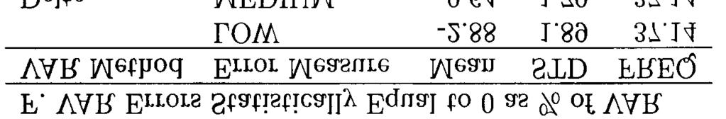
71

72

73

74

75 Table 3 Continued... Notes: For VAR at the l% confidence level, for two groups of option positions (from simulation 1), the table provides summary statistics on six methods for computing VAR using three measures of VAR error or percentage error. The first group of option positions are long in one of 70 foreign exchange call options; the second are short in the same call options. The options vary by moneyness and time to expiration. The VAR methods are Delta, Delta- Gamma-Delta (DGD), Delta-Gamma-Minimization (DGMin), Delta-Gamma Monte-Carlo (DGMC), Modified Grid Monte-Carlo (ModGridMC), and Monte Carlo with full repricing (Fu1lMC). For each group of option positions, the table reports the proportion (FREQ) for which VAR was overstated, understated, or statistically indistinguishable from zero. For positions classified as over- or under- stated, the Mean and Standard Deviation (STD) of overor under- statement are computed for three measures of error, LOW (an optimistic measure of error) MEDIUM (a less optimistic measure of error), and HIGH (a pessimistic measure of error). LOW, and HIGH are the endpoints of a 95% confidence interval for the amount of over- or under- statement. For positions classified as statistically indistinguishable from zero, LOW and HIGH are endpoints of a 95% confidence interval for VAR error. For all positions MEDIUM is always between LOW and HIGH, and measures error as the difference between a VAR estimate and Fu1lMC estimate or as the difference between a VAR estimate and Fu1lMC as a percentage of FullMC. A VAR estimate was classified as overstated if the 95% confidence interval for its error was bounded below by 0; it was classified as understated if the confidence interval for its error was bounded above by 0, and was statistically indistinguishable from 0 if the 95% confidence interval for its error contained 0. To rank the VAR methods two statistical loss functions are reported, Mean Absolute Error (MAE), and Root Mean Squared Error (RMSE). These loss functions were computed using an optimistic measure of error (LOW), a pessimistic measure (HIGH), and a middle range measure (MEDIUM). The loss function results in panel A are computed based on the levels of errors, the loss function results in panel B are computed based on the errors as a percent of true VAR. Details on the VAR methods are contained in section II; details on the confidence intervals are contained in appendix A; details on the option positions and statistical loss functions are contained in section V and appendix B. 72

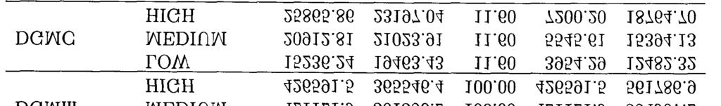
76