FEEG6017 lecture: The normal distribution, estimation, confidence intervals. Markus Brede,

Transcription

1 FEEG6017 lecture: The normal distribution, estimation, confidence intervals. Markus Brede,

2 The normal distribution The normal distribution is the classic "bell curve". We've seen that we can produce one by adding or averaging a large-enough group of random variates from any distribution. It can also be specified as a probability density function.

3 The normal distribution The normal distribution is central to statistical inference. A particular normal distribution is fully characterized by just two parameters: the mean, μ, and the standard deviation, σ. In other words, once you've said where the centre of the distribution is, and how wide it is, you've said all you can about it. The general shape of the curve is consistent.

4 The normal distribution

5 Standard normal distribution Because the normal distribution has this constant shape we can translate any instance of it into a standardized form. This is because of the scaling relations we discussed when we discussed the proof of the CLT. For each value, subtract the mean and divide by the standard deviation. This gives us the standard normal distribution which has μ = 0 and σ = 1 (red line on previous slide). Values on the standard normal indicate the number of standard deviations that an observation is above or below the mean. They're also called z-scores.

6 Areas under the normal curve The normal distribution's consistent shape is useful because we can say precise things about areas under the curve. It's a probability distribution so the area sums to 100%. 68% of the time the variate will be within plus or minus one standard deviation of the mean (i.e., a z-score between -1 and 1). 95% of variates will be within two standard deviations. 99.7% of variates will be within three standard deviations.

7 Areas under the normal curve

8 Variates from the normal distribution Suppose we have a normal distribution with a mean of 100 and a standard deviation of 10. We can reason about how unusual particular values are. For example, only 0.1% of cases will have a score higher than 130. Around 95% of cases will lie between 80 and 120. Conversely, only about 5% of cases will be more than 20 points away from % of cases will be between 100 and 110.

9 Z-tables In practice these days we use statistical calculators like R to figure out these areas under the normal curve. In the past, you had to look up a pre-computed "Z-table". Area remaining Positive Z- under the score curve to the right of this point

10 Notable z-scores A few useful z-scores to remember... Z = leaves 5% of the curve to the right. Z = 1.96 leaves 2.5% of the curve to the right. Z = leaves 0.5% of the curve to the right.

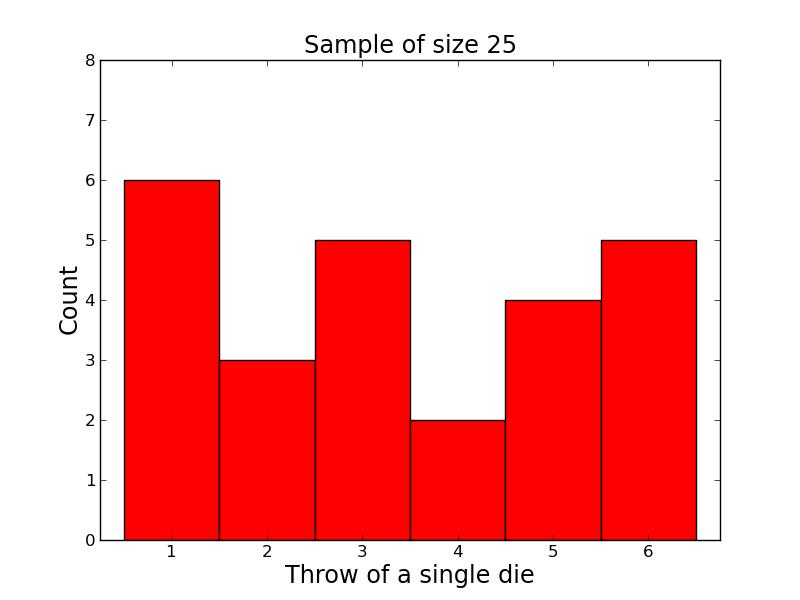
11 Thinking of a particular sample mean as a variate from a normal distribution Recall the uniform distribution of integers between 1 and 6 we get from throwing a single die. We found previously that if we repeatedly take samples of size N from that distribution, we end up with our collection of sample means being approximately normally distributed.

12

13 Sampling distribution of the mean What can we say about this approximately normal distribution of sample means? The mean is the same as the original population mean, i.e., 3.5 in this case. The standard deviation is the same as the original distribution's, scaled by 1 / sqrt(n), where N is the sample size. In the N=25 case, that's / sqrt(25) =

14 A note about why we're doing this Remember that in real cases nobody is interested in the green histogram for its own sake. If you really had the resources to collect 10,000 samples of size 25, you'd just call it one huge sample of 250,000. In the real case you get only your single sample of size 25, and you're trying to make inferences about the population based on just that. These computational experiments where we generate many such samples are attempts to stand back from that one-shot perspective.

15 A problem So it looks as though we're ready to draw conclusions about how unusual certain sample means might be. After all, we've got an approximately normal distribution (of sample means) and we know its mean and sd. But there's a problem: we're helping ourselves to information we wouldn't have in the real case. The original population's mean and standard deviation are typically exactly the things we're trying to find, not pre-given information.

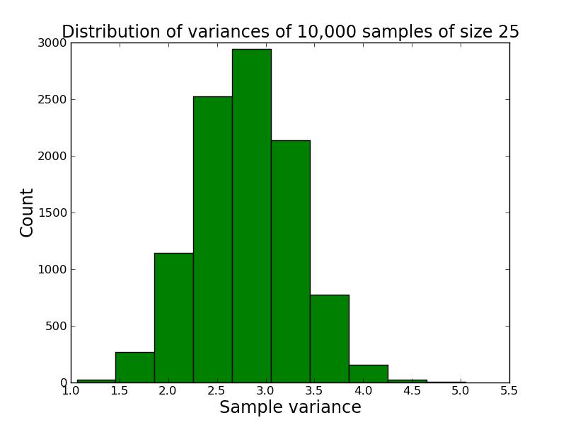
16 Sampling distribution of the variance We need to work with the only things we have, i.e., the properties of our sample. We know that the mean of our sample is a "good guess" for the mean of the population. What about the variance of our sample? We haven't systematically checked the relationship between sample variance and population variance yet. Let's take 10,000 samples of size 25, calculate the variance in each case, and consider the distribution of those sample variances.

17

18 Sampling distribution of the variance At first glance this all looks good. The variances of many samples of size 25 seem to be themselves roughly normally distributed and they seem to be zeroing in on the true value of But let's look more closely: for sample sizes between 2 and 10, we'll try collecting 10,000 samples and noting the average value of the calculated sample variance. Turns out there's a systematic problem of underestimation.

19

20 Biased and unbiased estimators The sample mean is an unbiased estimator of the population mean. This means that although our sample mean may be quite far from the true value, it's equally likely to be high or low. The sample variance is a biased estimator of the population variance. The sample variance will systematically underestimate the population variance, especially so for small sample sizes.

21 The sample variance and sample SD Bessel's correction is needed in order to find an unbiased estimator of the population variance. This means simply that we need to divide through by (N - 1) instead of N when calculating the variance and standard deviation. The underestimation happens because we're using the same small set of numbers to estimate both the mean and the variance.

22 Bessel's correction The Maths When we are estimating the variance with Bessel's correction we essentially calculate: By definition of variance we also have: i.e. E ( 1 n (x n 1 i=1 i x) 2 ) =E ( Hence: 1 n ((x n 1 i=1 i μ) ( x μ)) 2 ) 1 n ((x n i=1 i μ) ( x μ)) 2 = 1 n (x n i=1 i μ) 2 ( x μ) 2 n E ( i=1 ((x i μ) ( x μ)) 2 )= i=1 E ( 1 n (x n 1 i=1 i x) 2 ) = 1 n 1 ( n i=1 n E ((x i μ) 2 ) n E (( x μ) 2 ) V [ x i ] nv [ x])

23 Bessel's Maths (cont.) The xi are a random sample from a distribution with variance 2. Thus: V (xi)= 2. We also have: V [ x]=v [1/n i=1 n n x i ]=1/n 2 i=1 V [x i ]=σ 2 /n Back to the last expression from the last slide... E ( 1 n (x n 1 i=1 i x) 2 ) = 1 n 1 ( n i=1 = 1 n 1 (nσ2 nσ 2 /n) =σ 2 V [ x i ] nv [ x])

24 Calculating the two values in Python & R pylab.var(variablename) or pylab.std(variablename) will get you the population version, i.e.., the divisor is N. If you want the sample version (divisor = N-1) you can specify pylab.var(variablename, ddof=1) or pylab.std(variablename, ddof=1). In R, somewhat confusingly, the functions var(variablename) and sd(variablename) automatically assume the sample version, i.e., divisor = N-1. The good news: none of this matters with decent sample sizes.

25 A realistic case At last we're in a position to take a particular sample of size 25 and see how we could use it to reason about the population. For the sake of the exercise, we'll pretend that we don't already know the true values of the population mean and variance.

26

27 A realistic case Some output from Python... Mean of the sample is 3.4 Variance of the sample is 3.44 Sample variance, estimating pop variance, is SD of the sample is Sample SD, estimating pop SD, is So, based on our sample information, the best guess for the population mean is 3.4, and for the population standard deviation it's (Not bad guesses: true values are 3.5 and )

28 A realistic case We can place this information in a wider context. We know that our sample mean is "noisy", i.e., it's really drawn from an approximately normal distribution of possible sample means. Our best guess for that distribution is that its mean is 3.4 and its standard deviation is / sqrt(25) = That calculation gives us the standard error of the mean, i.e., the estimated standard deviation of the sampling distribution for the mean.

29 Confidence intervals If the sampling distribution of the mean is normally distributed, we can say something about how unlikely it is to get an extreme value from that distribution. We know, for example, that getting a z-score more extreme than ±3 only happens 0.3% of the time. Using our best estimates for the sampling distribution's mean and SD, that's the equivalent of saying that sample means outside the range of 3.4 ± (3 x 0.379) will only happen 0.3% of the time.

30 Confidence intervals A very handy z-score is 1.96, because it leaves exactly 2.5% of the distribution to the right. If we consider both edges of the normal distribution, that means that only 5% of the time will we get values more extreme than z = ±1.96. So, 95% of the time, we expect our sample mean to lie within the range 3.4 ± (1.96 x 0.379). That's between and

31 Confidence intervals Remember that 3.4 is our absolute best guess for the mean. (We don't know that the true value is 3.5.) But we also know that 3.4 is unlikely to be exactly right. We know that we're vulnerable to sampling error. If the mean of a particular sample is within ±1.96 standard errors of the population mean 95% of the time, we can also reverse this logic. We can conclude that 95% of the time, the true population mean is within ±1.96 standard errors of our sample mean.

32 Confidence intervals To see this in formulae: The Z-table tells us that with 95% probability we have 1.96< μ x s <1.96 Estimated standard deviation of sampling distribution, s0/sqrt(n) True population mean Sample mean Hence, with 95% probability we have: 1.96 s+ x<μ<1.96 s+ x i.e. with 95% probability the true mean is in x±1.96 s

33 Confidence intervals And that's all a confidence interval is. In this case, we would say that the 95% confidence interval for the true population mean is between and Note that the right answer, 3.5, is within that interval. Not guaranteed: 5% of the time, the real value will be outside the interval. Of course we won't know when! Confidence intervals can be calculated for different confidence levels (90%, 99%) with different z-scores, and can be calculated for quantities other than the mean.

34 Additional material David M. Lane's tutorials on the normal distribution and on sampling. A guide to reporting standard deviations and standard errors. The Python code used to produce simulations and graphs for this lecture: part 1 and part 2.