Chapter 6: The Normal Distribution

Transcription

1 Chapter 6: The Normal Distribution Diana Pell Section 6.1: Normal Distributions Note: Recall that a continuous variable can assume all values between any two given values of the variables. Many continuous variables have distributions that are bell-shaped, and these are called approximately normally distributed variables. If a random variable has a probability distribution whose graph is continuous, bell-shaped, and symmetric, it is called a normal distribution. The graph is called a normal distribution curve. 1

2 Summary of the Properties of the Theoretical Normal Distribution 1. A normal distribution curve is bell-shaped. 2. The mean, median, and mode are equal and are located at the center of the distribution. 3. A normal distribution curve is unimodal (i.e., it has only one mode). 4. The curve is symmetric about the mean. 5. The curve is continuous. 6. The curve never touches the x axis. 7. The total area under a normal distribution curve is equal to 1.00, or 100%. 8. The area under the part of a normal curve that lies within 1 standard deviation of the mean is approximately 0.68, or 68%; within 2 standard deviations, about 0.95, or 95%; and within 3 standard deviations, about 0.997, or 99.7%. 2

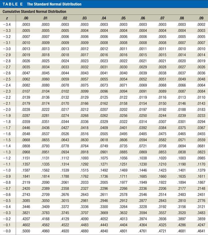
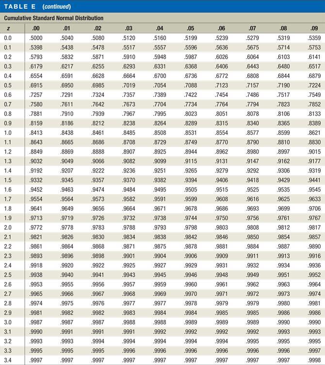
3 The standard normal distribution is a normal distribution with a mean of 0 and a standard deviation of 1. All normally distributed variables can be transformed into the standard normally distributed variable by using the formula for the standard score: z = value - mean standard deviation or z = X µ σ The z value or z score is actually the number of standard deviations that a particular X value is away from the mean. Finding the Area Under the Standard Normal Distribution Curve 3

4 Exercise 1. Find the area under the standard normal distribution curve. a) To the left of z = b) To the right of z = c) Between z = 1.62 and z = d) Between z = 0 and z = 1.77 e) To the right of z =

5 A Normal Distribution Curve as a Probability Distribution Curve Note: The area under the standard normal distribution curve can also be thought of as a probability or as the proportion of the population with a given characteristic. Exercise 2. Find the probability for each. (Assume this is a standard normal distribution.) a) P (0 < z < 2.35) b) P (z < 1.73) c) P (z > 1.98) Exercise 3. Find the z value that corresponds to the given area. a) b) 5

6 Exercise 4. Find the z value to the right of the mean so that a) 54.78% of the area under the distribution curve lies to the left of it. b) 82.12% of the area under the distribution curve lies to the right of it. Exercise 5. Many times in statistics it is necessary to see if a set of data values is approximately normally distributed. There are special techniques that can be used. One technique is to draw a histogram for the data and see if it is approximately bell-shaped. (Note: It does not have to be exactly symmetric to be bell-shaped.) The numbers of branches of the 50 top libraries are shown. a) Construct a frequency distribution for the data. 6

7 b) Construct a histogram for the data. c) Describe the shape of the histogram. d) Based on your answer to part (c), do you feel that the distribution is approximately normal? e) Find the mean and standard deviation for the data. f) What percent of the data values fall within 1 standard deviation of the mean? 7

8 g) What percent of the data values fall within 2 standard deviations of the mean? h) What percent of the data values fall within 3 standard deviations of the mean? i) How do your answers to parts (f), (g), and (h) compare to 68, 95, and 100%, respectively? j) Does your answer help support the conclusion you reached in part (d)? Explain. Section 6.2: Applications of the Normal Distribution 8

9 Suppose that the scores for a standardized test are normally distributed, have a mean of 100, and have a standard deviation of 15. Finding the Area Under Any Normal Curve 1. Draw a normal curve and shade the desired area. 2. Convert the values of X to z values, using the formula 3. Find the corresponding area using a table. z = X µ σ Exercise 6. An adult has on average 5.2 liters of blood. Assume the variable is normally distributed and has a standard deviation of 0.3. Find the percentage of people who have less than 5.4 liters of blood in their system. 9

10 Exercise 7. Each month, an American household generates an average of 28 pounds of newspaper for garbage or recycling. Assume the variable is approximately normally distributed and the standard deviation is 2 pounds. If a household is selected at random, find the probability of its generating a) Between 27 and 31 pounds per month b) More than 30.2 pounds per month Exercise 8. A desktop PC uses 120 watts of electricity per hour based on 4 hours of use per day. Assume the variable is approximately normally distributed and the standard deviation is 6. If 500 PCs are selected, approximately how many will use less than 106 watts of power? 10

11 Exercise 9. Newborn elephant calves usually weigh between 200 and 250 poundsuntil October 2006, that is. An Asian elephant at the Houston (Texas) Zoo gave birth to a male calf weighing in at a whopping 384 pounds! Mack (like the truck) is believed to be the heaviest elephant calf ever born at a facility accredited by the Association of Zoos and Aquariums. If, indeed, the mean weight for newborn elephant calves is 225 pounds with a standard deviation of 45 pounds, what is the probability of a newborn weighing at least 384 pounds? Assume that the weights of newborn elephants are normally distributed. Finding Data Values Given Specific Probabilities Formula for Finding the Value of a Normal Variable X X = z σ + µ Exercise 10. To qualify for a police academy, candidates must score in the top 10% on a general abilities test. Assume the test scores are normally distributed and the test has a mean of 200 and a standard deviation of 20. Find the lowest possible score to qualify. 11

12 Exercise 11. For a medical study, a researcher wishes to select people in the middle 60% of the population based on blood pressure. Assuming that blood pressure readings are normally distributed and the mean systolic blood pressure is 120 and the standard deviation is 8, find the upper and lower readings that would qualify people to participate in the study. Note: There are several ways statisticians check for normality. The easiest way is to draw a histogram for the data and check its shape. If the histogram is not approximately bell-shaped, then the data are not normally distributed. Skewness can be checked by using the Pearson coefficient (PC) of skewness also called Pearson s index of skewness. The formula is PC = 3( X median ) s If the index is greater than or equal to +1 or less than or equal to 1, it can be concluded that the data are significantly skewed. 12

13 Exercise 12. A survey of 18 high-tech firms showed the number of days inventory they had on hand. Determine if the data are approximately normally distributed. 13

14 Exercise 13. The data shown consist of the number of games played each year in the career of Baseball Hall of Famer Bill Mazeroski. Determine if the data are approximately normally distributed. 14

15 Section 6.3: The Central Limit Theorem A sampling distribution of sample means is a distribution using the means computed from all possible random samples of a specific size taken from a population. Sampling error is the difference between the sample measure and the corresponding population measure due to the fact that the sample is not a perfect representation of the population. Properties of the Distribution of Sample Means 1. The mean of the sample means will be the same as the population mean. 2. The standard deviation of the sample means will be smaller than the standard deviation of the population, and it will be equal to the population standard deviation divided by the square root of the sample size. Exercise 14. Suppose a professor gave an 8-point quiz to a small class of four students. The results of the quiz were 2, 6, 4, and 8. Assume that the four students constitute the population. 15

16 The Central Limit Theorem As the sample size n increases without limit, the shape of the distribution of the sample means taken with replacement from a population with mean µ and standard deviation s will approach a normal distribution. As previously shown, this distribution will have a mean and a standard deviation σ n Note: If the sample size is sufficiently large, the central limit theorem can be used to answer questions about sample means in the same manner that a normal distribution can be used to answer questions about individual values. The only difference is that a new formula must be used for the z values. It is z = X µ σ/ n It s important to remember two things when you use the central limit theorem: a) When the original variable is normally distributed, the distribution of the sample means will be normally distributed, for any sample size n. b) When the distribution of the original variable is not normal, a sample size of 30 or more is needed to use a normal distribution to approximate the distribution of the sample means. The larger the sample, the better the approximation will be. Exercise 15. A. C. Neilsen reported that children between the ages of 2 and 5 watch an average of 25 hours of television per week. Assume the variable is normally distributed and the standard deviation is 3 hours. If 20 children between the ages of 2 and 5 are randomly selected, find the probability that the mean of the number of hours they watch television will be greater than 26.3 hours. 16

17 Exercise 16. The average age of a vehicle registered in the United States is 8 years, or 96 months. Assume the standard deviation is 16 months. If a random sample of 36 vehicles is selected, find the probability that the mean of their age is between 90 and 100 months. Note: To gain information about an individual data value obtained from the population, use formula z = X µ X µ. To gain information about a sample mean, use formula z = σ Exercise 17. The average time spent by construction workers who work on weekends is 7.93 hours (over 2 days). Assume the distribution is approximately normal and has a standard deviation of 0.8 hour. a) Find the probability that an individual who works at that trade works fewer than 8 hours on the weekend. σ/ n 17

18 b) If a sample of 40 construction workers is randomly selected, find the probability that the mean of the sample will be less than 8 hours. The probability of selecting an individual construction worker who works less than 8 hours on a weekend is. The probability of selecting a random sample of 40 construction workers with a mean of less than 8 hours per week is. This difference of is due to the fact that the distribution of sample means is much less variable than the distribution of individual data values. The reason is that as the sample size increases, the standard deviation of the means decreases. 18

19 19

20 20