6.2.1 Linear Transformations
|
|
|
- Jemimah Hutchinson
- 6 years ago
- Views:
Transcription
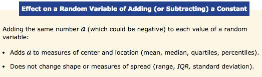
 a constant: Adding the same number a (either positive, zero, or negative) to each observation: Adds a to measures of center and location (mean, median, quartiles, percentiles).")
1 6.2.1 Linear Transformations In Chapter 2, we studied the effects of transformations on the shape, center, and spread of a distribution of data. Recall what we discovered: 1. Adding (or subtracting) a constant: Adding the same number a (either positive, zero, or negative) to each observation: Adds a to measures of center and location (mean, median, quartiles, percentiles). Does not change shape or measures of spread (range, IQR, standard deviation). 2. Multiplying (or dividing) each observation by a constant b (positive, negative, or zero): Multiplies (divides) measures of center and location (mean, median, quartiles, percentiles) by b. Multiplies (divides) measures of spread (range, IQR, standard deviation) by b. Does not change the shape of the distribution. Effect of multiplying or dividing by a constant Let s start with a simple example of a discrete random variable. Pete s Jeep Tours offers a popular half- day trip in a tourist area. There must be at least 2 passengers for the trip to run, and the vehicle will hold up to 6 passengers. The number of passengers X on a randomly selected day has the following probability distribution. The mean of X is: The variance is: The standard deviation is:

2 Example Pete s Jeep Tours Multiplying a random variable by a constant Pete charges $150 per passenger. Let C = the total amount of money that Pete collects on a randomly selected trip. Because the amount of money Pete collects from the trip is just $150 times the number of passengers, we can write C = 150X. From the probability distribution of X, we can see that the chance of having two people (X = 2) on the trip is In that case, C =(150)(2) = 300. So one possible value of C is $300, and its corresponding probability is If X = 3, then C = (150)(3) = 450, and the corresponding probability is Thus, the probability distribution of C is: The mean of C is μ C = Σ c i p i = (300)(0.15) + (450)(0.25) + + (900)(0.05) = On average, Pete will collect a total of $ from the half- day trip. The variance of C is: So the standard deviation of C is: In the previous example, the random variable C was obtained by multiplying the values of our earlier random variable X by 150. To understand the effect of multiplying by a constant, let s compare the probability distributions of these two random variables. Shape: The two probability distributions have the same shape. Center: The mean of X is µ X = The mean of C is µ C = , which is (150)(3.75).That is, µ C = 150µ X. Spread: The standard deviation of X is σ X = The standard deviation of C is σ C = 163.5, which is (150)(1.090). That is, σ C = 150σ X.

, then C = 300 and V = 200. From the probability distribution of C, the chance that this happens is 0.15.")
3 As with data, if we multiply a random variable by a negative constant b, our common measures of spread are multiplied by b. Example Pete s Jeep Tours Effect of adding or subtracting a constant It costs Pete $100 to buy permits, gas, and a ferry pass for each half- day trip. The amount of profit V that Pete makes from the trip is the total amount of money C that he collects from passengers minus $100. That is, V = C 100. If Pete has only two passengers on the trip (X = 2), then C = 300 and V = 200. From the probability distribution of C, the chance that this happens is So the smallest possible value of V is $200; its corresponding probability is If X = 3, then C = 450 and V = 350, and the corresponding probability is The probability distribution of V is: The mean of V is μ V = Σv i p i = (200)(0.15) + (350)(0.25) +, + (800)(0.05) = On average, Pete will make a profit of $ from the trip. The variance of V is: So the standard deviation of V is:
4
5 CHECK YOUR UNDERSTANDING A large auto dealership keeps track of sales made during each hour of the day. Let X = the number of cars sold during the first hour of business on a randomly selected Friday. Based on previous records, the probability distribution of X is as follows: The random variable X has mean µ X = 1.1 and standard deviation σ X = Suppose the dealership s manager receives a $500 bonus from the company for each car sold. Let Y = the bonus received from car sales during the first hour on a randomly selected Friday. Find the mean and standard deviation of Y. 2. To encourage customers to buy cars on Friday mornings, the manager spends $75 to provide coffee and doughnuts. The manager s net profit T on a randomly selected Friday is the bonus earned minus this $75. Find the mean and standard deviation of T.

6 Putting it all together: Adding/subtracting and multiplying/dividing What happens if we transform a random variable by both adding or subtracting a constant and multiplying or dividing by a constant? Let s consider Pete s Jeep Tours again. We could have gone directly from the number of passengers X on a randomly selected jeep tour to Pete s profit V with the equation V = 150X 100 or, equivalently, V = X. This linear transformation of the random variable X includes both of the transformations that we performed earlier: (1) multiplying by 150 and (2) subtracting 100. (In general, a linear transformation can be written in the form Y = a + bx, where a and b are constants.) The net effect of this sequence of transformations is as follows: Shape: Neither transformation changes the shape of the probability distribution. Center: The mean of X is multiplied by 150 and then decreased by 100; that is, μ V = 150μ X 100 = μ X. Spread: The standard deviation of X is multiplied by 150 and is unchanged by the subtraction: σ V = 150σ X. For the linear transformationv = X, it would not be correct to apply the transformations in the reverse order: subtract 100 and then multiply by 150. Doing so would yield the same standard deviation but a different (wrong) mean. This logic generalizes to any linear transformation. Can you see why this is called a "linear" transformation? The equation describing the sequence of transformations has the form Y = a + bx, which you should recognize as a linear equation.
7 Example The Baby and the Bathwater Linear transformations One brand of bathtub comes with a dial to set the water temperature. When the babysafe setting is selected and the tub is filled, the temperature X of the water follows a normal distribution with a mean of 34 C and a standard deviation of 2 C. (a) Define the random variable Y to be the water temperature in degrees Fahrenheit (recall that ) when the dial is set on babysafe. Find the mean and standard deviation of Y. (b) According to Babies R Us, the temperature of a baby s bathwater should be between 90 F and 100 F. Find the probability that the water temperature on a randomly selected day when the babysafe setting is used meets the babies r us recommendation. Show your work.


8 6.2.2 Combining Random Variables Example Put a Lid on It! When one random variable isn t enough If we buy a large drink at a fast- food restaurant and grab a large- sized lid, we assume that the lid will fit snugly on the cup. Usually, it does. Sometimes, though, the lid is a bit too small or too large to fit securely. Why does this happen? Even though the large cups are made to be identical in size, the width actually varies slightly from cup to cup. In fact, the diameter of a randomly selected large drink cup is a random variable (call it C) that has a particular probability distribution. Likewise, the diameter of a randomly selected large lid (call it L) is a random variable with its own probability distribution. For a lid to fit on a cup, the value of L has to be bigger than the value of C, but not too much bigger. To find the probability that the lid fits, we need to know more about what happens when we combine these two random variables. Sums of random variables Earlier, we examined the probability distribution for the random variable X = the number of passengers on a randomly selected half- day trip with Pete s Jeep Tours. Here s a brief recap: Pete s sister Erin, who lives near a tourist area in another part of the country, is impressed by the success of Pete s business. She decides to join the business, running tours on the same days as Pete in her slightly smaller vehicle, under the name Erin s Adventures. After a year of steady bookings, Erin discovers that the number of passengers Y on her half- day tours has the following probability distribution. Below is a histogram of this probability distribution.

9 How many total passengers T can Pete and Erin expect to have on their tours on a randomly selected day? Since Pete averages μ X = 3.75 passengers per trip and Erin averages μ Y = 3.10 passengers per trip, they will average a total of μ T = = 6.85 passengers per day. We can generalize this result for any two random variables as follows: if T = X + Y, then μ T = μ X + μ Y. In other words, the expected value (mean) of the sum of two random variables is equal to the sum of their expected values (means). How much variability is there in the total number of passengers who go on Pete s and Erin s tours on a randomly chosen day? Let s think about the possible values of T = X + Y.The number of passengers X on Pete s tour is between 2 and 6, and the number of passengers Y on Erin s tour is between 2 and 5. So the total number of passengers T is between 4 and 11. Thus, the range of T is 11 4 = 7. How is this value related to the ranges of X and Y? The range of X is 4 and the range of Y is 3, so range of T = range of X + range of Y That is, there s more variability in the values of T than in the values of X or Y alone. This makes sense, because the variation in X and the variation in Y both contribute to the variation in T. What about the standard deviation σ T? If we had the probability distribution of the random variable T, then we could calculate σ T. Let s try to construct this probability distribution starting with the smallest possible value, T = 4. The only way to get a total of 4 passengers is if Pete has X = 2 passengers and Erin has Y = 2 passengers. We know that P(X = 2) = 0.15 and that P(Y = 2) = 0.3. If the two events X = 2 and Y = 2 are independent, then we can multiply these two probabilities. Otherwise, we re stuck. In fact, we can t calculate the probability for any value of T unless X and Y are independent random variables. Independent Random Variables - If knowing whether any event involving X alone has occurred tells us nothing about the occurrence of any event involving Y alone, and vice versa, then X and Y are independent random variables. Probability models often assume independence when the random variables describe outcomes that appear unrelated to each other. You should always ask whether the assumption of independence seems reasonable. For instance, it s reasonable to treat the random variables X = number of passengers on Pete s trip and Y = number of passengers on Erin s trip on a randomly chosen day as independent, since the siblings operate their trips in different parts of the country. Now we can calculate the probability distribution of the total number of passengers that day.
10 Example Pete s Jeep Tours and Erin s Adventures Sum of two random variables Let T = X + Y, as before. Assume that X and Y are independent random variables. We ll begin by considering all the possible combinations of values of X and Y. Now we can construct the probability distribution by adding the probabilities for each possible value of T. For instance, P(T = 6) = = You can check that the probabilities add to 1. A histogram of the probability distribution is shown in Figure The mean of T is μ T = Σt i p i = (4)(0.045) + (5)(0.135) + + (11)(0.005) = Recall that μ X = 3.75 and μ Y = Our calculation confirms that μ T = μ X + μ Y = = 6.85

11 What about the variance of T? It s Now and. Do you see the relationship? Variances add! To find the standard deviation of T, take the square root of the variance As the preceding example illustrates, when we add two independent random variables, their variances add. Standard deviations do not add. For Pete s and Erin s passenger totals, σ X + σ Y = = This is very different from σ Y =
12 Example SAT Scores The role of independence A college uses SAT scores as one criterion for admission. Experience has shown that the distribution of SAT scores among its entire population of applicants is such that PROBLEM: What are the mean and standard deviation of the total score X + Yamong students applying to this college?
13 Example Pete s and Erin s Tours Rules for adding random variables Earlier, we defined X = the number of passengers on Pete s trip, Y = the number of passengers on Erin s trip, and C = the amount of money that Pete collects on a randomly selected day. We also found the means and standard deviations of these variables: PROBLEM: (a) Erin charges $175 per passenger for her trip. Let G = the amount of money that she collects on a randomly selected day. Find the mean and standard deviation of G. (b) Calculate the mean and the standard deviation of the total amount that Pete and Erin collect on a randomly chosen day.
14 We can extend our rules for adding random variables to situations involving repeated observations from the same chance process. For instance, suppose a gambler plays two games of roulette, each time placing a $1 bet on either red or black. What can we say about his total gain (or loss) from playing two games? Earlier, we showed that if X = the amount gained on a single $1 bet on red or black, then μ X = $0.05 and σ X = $1.00. Since we re interested in the player s total gain over two games, we ll define X 1 as the amount he gains from the first game and X 2 as the amount he gains from the second game. Then, his total gain T = X 1 + X 2. Both X 1 and X 2 have the same probability distribution as X and, therefore, the same mean ( $0.05) and standard deviation ($1.00). The player s expected gain in two games is Since the result of one game has no effect on the result of the other game, X 1 and X 2 are independent random variables. As a result, and the standard deviation of the player s total gain is
15 CHECK YOUR UNDERSTANDING A large auto dealership keeps track of sales and lease agreements made during each hour of the day. Let X = the number of cars sold and Y = the number of cars leased during the first hour of business on a randomly selected Friday. Based on previous records, the probability distributions of X and Y are as follows: Define T = X + Y. 1. Find and interpret µ T, 2. Compute σ T assuming that X and Y are independent. Show your work. 3. The dealership s manager receives a $500 bonus for each car sold and a $300 bonus for each car leased. Find the mean and standard deviation of the manager s total bonus B. Show your work.

16 Differences of random variables Now that we ve examined sums of random variables, it s time to investigate the difference of two random variables. Let s start by looking at the difference in the number of passengers that Pete and Erin have on their tours on a randomly selected day, D = X Y. Since Pete averages μ X = 3.75 passengers per trip and Erin averages μ Y = 3.10 passengers per trip, the average difference is μ D = = 0.65 passengers. That is, Pete averages 0.65 more passengers per day than Erin does. We can generalize this result for any two random variables as follows: if D = X Y, then μ D = μ X μ Y. In other words, the expected value (mean) of the difference of two random variables is equal to the difference of their expected values (means). The order of subtraction is important. If we had defined D = Y X, then µ D = µ Y µ X = = In other words, Erin averages 0.65 fewer passengers than Pete does on a randomly chosen day. Earlier, we saw that the variance of the sum of two independent random variables is the sum of their variances. Can you guess what the variance of the difference of two independent random variables will be? (If you were thinking something like the difference of their variances, think again!) Let s return to the jeep tours scenario. On a randomly selected day, the number of passengers X on Pete s tour is between 2 and 6,and the number of passengers Y on Erin s tour is between 2 and 5. So the difference in the number of passengers D = X Y is between 3 and 4. Thus, the range of D is 4 ( 3) = 7. How is this value related to the ranges of X and Y? The range of X is 4 and the range of Y is 3, so range of D = range of X + range of Y As with sums of random variables, there s more variability in the values of the difference D than in the values of X or Y alone. This should make sense, because the variation in X and the variation in Y both contribute to the variation in D. If you follow the process we used earlier with the random variable T = X + Y, you can build the probability distribution of D = X Y and confirm that (1) µ D = µ X µ Y = = 0.65 (2) (3) Result 2 shows that, just like with addition, when we subtract two independent random variables, variances add.

17 Example Pete s Jeep Tours and Erin s Adventures Difference of random variables Difference of random variables We have defined several random variables related to Pete s and Erin s tour businesses. For a randomly selected day, X = number of passengers on Pete s trip C = amount of money that Pete collects Y = number of passengers on Erin s trip G = amount of money that Erin collects Here are the means and standard deviations of these random variables: PROBLEM: Calculate the mean and the standard deviation of the difference D = C G in the amounts that Pete and Erin collect on a randomly chosen day. Interpret each value in context.
18 CHECK YOUR UNDERSTANDING A large auto dealership keeps track of sales and lease agreements made during each hour of the day. Let X = the number of cars sold and Y = the number of cars leased during the first hour of business on a randomly selected Friday. Based on previous records, the probability distributions of X and Y are as follows: Define D = X Y. 1. Find and interpret µ D 2. Compute σ D assuming that X and Y are independent. Show your work. 3. The dealership s manager receives a $500 bonus for each car sold and a $300 bonus for each car leased. Find the mean and standard deviation of the difference in the manager s bonus for cars sold and leased. Show your work.
 shows the results. The random variable X is N(3, 0.9) and the random variable Y is N(1, 1.2).")
 came from adding and subtracting the values of X and Y for the 1000 randomly generated observations from each distribution.")
19 6.2.3 Combining Normal Random Variables Example A Computer Simulation Sums and Differences of Normal random variables We used Fathom software to simulate taking independent SRSs of 1000 observations from each of two Normally distributed random variables, X and Y. Figure (a) shows the results. The random variable X is N(3, 0.9) and the random variable Y is N(1, 1.2).What do we know about the sum and difference of these two random variables? The histograms in Figure (b) came from adding and subtracting the values of X and Y for the 1000 randomly generated observations from each distribution. Let s summarize what we see: As the previous example illustrates, any sum or difference of independent Normal random variables is also Normally distributed. The mean and standard deviation of the resulting Normal distribution can be found using the appropriate rules for means and variances.

20 Example Give Me Some Sugar Sums of Normal random variables Mr. Starnes likes sugar in his hot tea. From experience, he needs between 8.5 and 9 grams of sugar in a cup of tea for the drink to taste right. While making his tea one morning, Mr. Starnes adds four randomly selected packets of sugar. Suppose the amount of sugar in these packets follows a Normal distribution with mean 2.17 grams and standard deviation 0.08 grams. STATE: What s the probability that Mr. Starnes s tea tastes right? PLAN: Let X = the amount of sugar in a randomly selected packet. Then X 1 = amount of sugar in Packet 1, X 2 = amount of sugar in Packet 2, X 3 = amount of sugar in Packet 3,and X 4 = amount of sugar in Packet 4. Each of these random variables has a normal distribution with mean 2.17 grams and standard deviation 0.08 grams. We re interested in the total amount of sugar that Mr. Starnes puts in his tea, which is given by T = X 1 +X 2 + X 3 + X 4. Our goal is to find P(8.5 T 9). DO: The random variable T is a sum of four independent Normal random variables. So T follows a normal distribution with mean and variance The standard deviation of T is We want to find the probability that the total amount of sugar in Mr. Starnes s tea is between 8.5 and 9 grams. The figure below shows this probability as the area under a normal curve. To find this area, we can standardize and use the z- table: Then P( 1.13 Z 2.00) = = CONCLUDE: There s about an 85% chance that Mr. Starnes s tea will taste right. Using normalcdf (8.5, 9, 8.68, 0.16) yields P(8.5 T 9) =
21 Example Put a Lid on It! Differences of Normal random variables The diameter C of a randomly selected large drink cup at a fast- food restaurant follows a Normal distribution with a mean of 3.96 inches and a standard deviation of 0.01 inches. The diameter L of a randomly selected large lid at this restaurant follows a Normal distribution with mean 3.98 inches and standard deviation 0.02 inches. For a lid to fit on a cup, the value of L has to be bigger than the value of C, but not by more than 0.06 inches. STATE: What s the probability that a randomly selected large lid will fit on a randomly chosen large drink cup? PLAN: We ll define the random variable D = L C to represent the difference between the lid s diameter and the cup s diameter. Our goal is to find P(O < D 0.06). Do: The random variable D is the difference of two independent Normal random variables. So D follows a normal distribution with mean and variance μ D = μ L μ C = = 0.02 The standard deviation of D is We want to find the probability that the difference D is between 0 and 0.06 inches. The figure below shows this probability as the area under a normal curve. to find this area,we can standardize and use a z- table: ***Using normalcdf (0, 0.06, 0.02, ) yields P(0 < D 0.06) = Then P( 0.89 Z 1.79) = =
22 CONCLUDE: There s about a 78% chance that a randomly selected large lid will fit on a randomly chosen large drink cup at this fast- food restaurant. Roughly 22% of the time, the lid won t fit. This seems like an unreasonably high chance of getting a lid that doesn t fit. Maybe the restaurant should find a new supplier! Learn Simulating with randnorm
Section 6.2 Transforming and Combining Random Variables. Linear Transformations
 Section 6.2 Transforming and Combining Random Variables Linear Transformations In Section 6.1, we learned that the mean and standard deviation give us important information about a random variable. In
EDCC charges $50 per credit. Let T = tuition charge for a randomly-selected fulltime student. T = 50X. Tuit. T $600 $650 $700 $750 $800 $850 $900
 Chapter 7 Random Variables n 7.1 Discrete and Continuous Random Variables n 6.2 n Example: El Dorado Community College El Dorado Community College considers a student to be full-time if he or she is taking
CHAPTER 6 Random Variables
 CHAPTER 6 Random Variables 6.2 Transforming and Combining Random Variables The Practice of Statistics, 5th Edition Starnes, Tabor, Yates, Moore Bedford Freeman Worth Publishers Transforming and Combining
Chapter 6: Random Variables
 Chapter 6: Random Variables Section 6.2 The Practice of Statistics, 4 th edition For AP* STARNES, YATES, MOORE Chapter 6 Random Variables 6.1 Discrete and Continuous Random Variables 6.2 6.3 Binomial and
Chapter 6: Random Variables
 Chapter 6: Random Variables Section 6.2 The Practice of Statistics, 4 th edition For AP* STARNES, YATES, MOORE Chapter 6 Random Variables 6.1 Discrete and Continuous Random Variables 6.2 6.3 Binomial and
SECTION 6.2 (DAY 1) TRANSFORMING RANDOM VARIABLES NOVEMBER 16 TH, 2017
 TRANSFORMING RANDOM VARIABLES NOVEMBER 16 TH, 2017") SECTION 6.2 (DAY 1) TRANSFORMING RANDOM VARIABLES NOVEMBER 16 TH, 2017 TODAY S OBJECTIVES Describe the effects of transforming a random variable by: adding or subtracting a constant multiplying or dividing
SECTION 6.2 (DAY 1) TRANSFORMING RANDOM VARIABLES NOVEMBER 16 TH, 2017 TODAY S OBJECTIVES Describe the effects of transforming a random variable by: adding or subtracting a constant multiplying or dividing
Section 7.4 Transforming and Combining Random Variables (DAY 1)
") Section 7.4 Learning Objectives (DAY 1) After this section, you should be able to DESCRIBE the effect of performing a linear transformation on a random variable (DAY 1) COMBINE random variables and CALCULATE
Section 7.4 Learning Objectives (DAY 1) After this section, you should be able to DESCRIBE the effect of performing a linear transformation on a random variable (DAY 1) COMBINE random variables and CALCULATE
Chapter 6: Random Variables
 Chapter 6: Random Variables Section 6. The Practice of Statistics, 4 th edition For AP* STARNES, YATES, MOORE Chapter 6 Random Variables 6.1 Discrete and Continuous Random Variables 6. 6.3 Binomial and
AP Stats ~ Lesson 6B: Transforming and Combining Random variables
 AP Stats ~ Lesson 6B: Transforming and Combining Random variables OBJECTIVES: DESCRIBE the effects of transforming a random variable by adding or subtracting a constant and multiplying or dividing by a
CHAPTER 6 Random Variables
 CHAPTER 6 Random Variables 6.2 Transforming and Combining Random Variables The Practice of Statistics, 5th Edition Starnes, Tabor, Yates, Moore Bedford Freeman Worth Publishers 6.2 Reading Quiz (T or F)
AP Statistics Chapter 6 - Random Variables
 AP Statistics Chapter 6 - Random 6.1 Discrete and Continuous Random Objective: Recognize and define discrete random variables, and construct a probability distribution table and a probability histogram
Honors Statistics. 3. Review OTL C6#3. 4. Normal Curve Quiz. Chapter 6 Section 2 Day s Notes.notebook. May 02, 2016.
 Honors Statistics Aug 23-8:26 PM 3. Review OTL C6#3 4. Normal Curve Quiz Aug 23-8:31 PM 1 May 1-9:09 PM Apr 28-10:29 AM 2 27, 28, 29, 30 Nov 21-8:16 PM Working out Choose a person aged 19 to 25 years at
Honors Statistics. Daily Agenda
 Honors Statistics Daily Agenda 1. Review OTL C6#5 2. Quiz Section 6.1 A-Skip 35, 39, 40 Crickets The length in inches of a cricket chosen at random from a field is a random variable X with mean 1.2 inches
Stats CH 6 Intro Activity 1
 Stats CH 6 Intro Activit 1 1. Purpose can ou tell the difference between bottled water and tap water? You will drink water from 3 samples. 1 of these is bottled water.. You must test them in the following
Honors Statistics. Daily Agenda
 Honors Statistics Aug 23-8:26 PM Daily Agenda 1. Review OTL C6#4 Chapter 6.2 rules for means and variances Aug 23-8:31 PM 1 Nov 21-8:16 PM Working out Choose a person aged 19 to 25 years at random and
Probability & Sampling The Practice of Statistics 4e Mostly Chpts 5 7
 Probability & Sampling The Practice of Statistics 4e Mostly Chpts 5 7 Lew Davidson (Dr.D.) Mallard Creek High School Lewis.Davidson@cms.k12.nc.us 704-786-0470 Probability & Sampling The Practice of Statistics
Binomial Random Variable - The count X of successes in a binomial setting
 6.3.1 Binomial Settings and Binomial Random Variables What do the following scenarios have in common? Toss a coin 5 times. Count the number of heads. Spin a roulette wheel 8 times. Record how many times
HHH HHT HTH THH HTT THT TTH TTT
 AP Statistics Name Unit 04 Probability Period Day 05 Notes Discrete & Continuous Random Variables Random Variable: Probability Distribution: Example: A probability model describes the possible outcomes
4.2 Probability Distributions
 4.2 Probability Distributions Definition. A random variable is a variable whose value is a numerical outcome of a random phenomenon. The probability distribution of a random variable tells us what the
Part 1 In which we meet the law of averages. The Law of Averages. The Expected Value & The Standard Error. Where Are We Going?
 1 The Law of Averages The Expected Value & The Standard Error Where Are We Going? Sums of random numbers The law of averages Box models for generating random numbers Sums of draws: the Expected Value Standard
Chapter 6: Random Variables
 Chapter 6: Random Variables Section 6.1 Discrete and Continuous Random Variables The Practice of Statistics, 4 th edition For AP* STARNES, YATES, MOORE Chapter 6 Random Variables 6.1 Discrete and Continuous
MA 1125 Lecture 14 - Expected Values. Wednesday, October 4, Objectives: Introduce expected values.
 MA 5 Lecture 4 - Expected Values Wednesday, October 4, 27 Objectives: Introduce expected values.. Means, Variances, and Standard Deviations of Probability Distributions Two classes ago, we computed the
Solutions for practice questions: Chapter 15, Probability Distributions If you find any errors, please let me know at
 Solutions for practice questions: Chapter 15, Probability Distributions If you find any errors, please let me know at mailto:msfrisbie@pfrisbie.com. 1. Let X represent the savings of a resident; X ~ N(3000,
7 THE CENTRAL LIMIT THEOREM
 CHAPTER 7 THE CENTRAL LIMIT THEOREM 373 7 THE CENTRAL LIMIT THEOREM Figure 7.1 If you want to figure out the distribution of the change people carry in their pockets, using the central limit theorem and
CHAPTER 6 Random Variables
 CHAPTER 6 Random Variables 6.1 Discrete and Continuous Random Variables The Practice of Statistics, 5th Edition Starnes, Tabor, Yates, Moore Bedford Freeman Worth Publishers Discrete and Continuous Random
STAT Chapter 6 The Standard Deviation (SD) as a Ruler and The Normal Model
 as a Ruler and The Normal Model") STAT 203 - Chapter 6 The Standard Deviation (SD) as a Ruler and The Normal Model In Chapter 5, we introduced a few measures of center and spread, and discussed how the mean and standard deviation are good
STAT 203 - Chapter 6 The Standard Deviation (SD) as a Ruler and The Normal Model In Chapter 5, we introduced a few measures of center and spread, and discussed how the mean and standard deviation are good
6.1 Discrete & Continuous Random Variables. Nov 4 6:53 PM. Objectives
 6.1 Discrete & Continuous Random Variables examples vocab Objectives Today we will... - Compute probabilities using the probability distribution of a discrete random variable. - Calculate and interpret
STAT Chapter 6 The Standard Deviation (SD) as a Ruler and The Normal Model
 as a Ruler and The Normal Model") STAT 203 - Chapter 6 The Standard Deviation (SD) as a Ruler and The Normal Model In Chapter 5, we introduced a few measures of center and spread, and discussed how the mean and standard deviation are good
STAT 203 - Chapter 6 The Standard Deviation (SD) as a Ruler and The Normal Model In Chapter 5, we introduced a few measures of center and spread, and discussed how the mean and standard deviation are good
Making Sense of Cents
 Name: Date: Making Sense of Cents Exploring the Central Limit Theorem Many of the variables that you have studied so far in this class have had a normal distribution. You have used a table of the normal
CH 5 Normal Probability Distributions Properties of the Normal Distribution
 Properties of the Normal Distribution Example A friend that is always late. Let X represent the amount of minutes that pass from the moment you are suppose to meet your friend until the moment your friend
Example - Let X be the number of boys in a 4 child family. Find the probability distribution table:
 Chapter7 Probability Distributions and Statistics Distributions of Random Variables tthe value of the result of the probability experiment is a RANDOM VARIABLE. Example - Let X be the number of boys in
BIOL The Normal Distribution and the Central Limit Theorem
 BIOL 300 - The Normal Distribution and the Central Limit Theorem In the first week of the course, we introduced a few measures of center and spread, and discussed how the mean and standard deviation are
Math 2311 Bekki George Office Hours: MW 11am to 12:45pm in 639 PGH Online Thursdays 4-5:30pm And by appointment
 Math 2311 Bekki George bekki@math.uh.edu Office Hours: MW 11am to 12:45pm in 639 PGH Online Thursdays 4-5:30pm And by appointment Class webpage: http://www.math.uh.edu/~bekki/math2311.html Math 2311 Class
4.1 Probability Distributions
 Probability and Statistics Mrs. Leahy Chapter 4: Discrete Probability Distribution ALWAYS KEEP IN MIND: The Probability of an event is ALWAYS between: and!!!! 4.1 Probability Distributions Random Variables
Biostatistics and Design of Experiments Prof. Mukesh Doble Department of Biotechnology Indian Institute of Technology, Madras
 Biostatistics and Design of Experiments Prof. Mukesh Doble Department of Biotechnology Indian Institute of Technology, Madras Lecture - 05 Normal Distribution So far we have looked at discrete distributions
Chapter 7. Random Variables
 Chapter 7 Random Variables Making quantifiable meaning out of categorical data Toss three coins. What does the sample space consist of? HHH, HHT, HTH, HTT, TTT, TTH, THT, THH In statistics, we are most
Have you ever wondered whether it would be worth it to buy a lottery ticket every week, or pondered on questions such as If I were offered a choice
 Section 8.5: Expected Value and Variance Have you ever wondered whether it would be worth it to buy a lottery ticket every week, or pondered on questions such as If I were offered a choice between a million
Example - Let X be the number of boys in a 4 child family. Find the probability distribution table:
 Chapter8 Probability Distributions and Statistics Section 8.1 Distributions of Random Variables tthe value of the result of the probability experiment is a RANDOM VARIABLE. Example - Let X be the number
Data that can be any numerical value are called continuous. These are usually things that are measured, such as height, length, time, speed, etc.
 Chapter 8 Measures of Center Data that can be any numerical value are called continuous. These are usually things that are measured, such as height, length, time, speed, etc. Data that can only be integer
Expected Value of a Random Variable
 Knowledge Article: Probability and Statistics Expected Value of a Random Variable Expected Value of a Discrete Random Variable You're familiar with a simple mean, or average, of a set. The mean value of
Variance, Standard Deviation Counting Techniques
 Variance, Standard Deviation Counting Techniques Section 1.3 & 2.1 Cathy Poliak, Ph.D. cathy@math.uh.edu Department of Mathematics University of Houston 1 / 52 Outline 1 Quartiles 2 The 1.5IQR Rule 3 Understanding
STAT 201 Chapter 6. Distribution
 STAT 201 Chapter 6 Distribution 1 Random Variable We know variable Random Variable: a numerical measurement of the outcome of a random phenomena Capital letter refer to the random variable Lower case letters
Normal Model (Part 1)
") Normal Model (Part 1) Formulas New Vocabulary The Standard Deviation as a Ruler The trick in comparing very different-looking values is to use standard deviations as our rulers. The standard deviation
Normal Model (Part 1) Formulas New Vocabulary The Standard Deviation as a Ruler The trick in comparing very different-looking values is to use standard deviations as our rulers. The standard deviation
+ Chapter 7. Random Variables. Chapter 7: Random Variables 2/26/2015. Transforming and Combining Random Variables
 + Chapter 7: Random Variables Section 7.1 Discrete and Continuous Random Variables The Practice of Statistics, 4 th edition For AP* STARNES, YATES, MOORE + Chapter 7 Random Variables 7.1 7.2 7.2 Discrete
= 0.35 (or ˆp = We have 20 independent trials, each with probability of success (heads) equal to 0.5, so X has a B(20, 0.5) distribution.
 equal to 0.5, so X has a B(20, 0.5) distribution.") Chapter 5 Solutions 51 (a) n = 1500 (the sample size) (b) The Yes count seems like the most reasonable choice, but either count is defensible (c) X = 525 (or X = 975) (d) ˆp = 525 1500 = 035 (or ˆp = 975
Chapter 5 Solutions 51 (a) n = 1500 (the sample size) (b) The Yes count seems like the most reasonable choice, but either count is defensible (c) X = 525 (or X = 975) (d) ˆp = 525 1500 = 035 (or ˆp = 975
Chapter 6: Random Variables
 Chapter 6: Random Variables Section 6.3 The Practice of Statistics, 4 th edition For AP* STARNES, YATES, MOORE Chapter 6 Random Variables 6.1 Discrete and Continuous Random Variables 6.2 Transforming and
Both the quizzes and exams are closed book. However, For quizzes: Formulas will be provided with quiz papers if there is any need.
 Both the quizzes and exams are closed book. However, For quizzes: Formulas will be provided with quiz papers if there is any need. For exams (MD1, MD2, and Final): You may bring one 8.5 by 11 sheet of
Sampling Distributions
 AP Statistics Ch. 7 Notes Sampling Distributions A major field of statistics is statistical inference, which is using information from a sample to draw conclusions about a wider population. Parameter:
STA Module 3B Discrete Random Variables
 STA 2023 Module 3B Discrete Random Variables Learning Objectives Upon completing this module, you should be able to 1. Determine the probability distribution of a discrete random variable. 2. Construct
8.2 The Standard Deviation as a Ruler Chapter 8 The Normal and Other Continuous Distributions 8-1
 8.2 The Standard Deviation as a Ruler Chapter 8 The Normal and Other Continuous Distributions For Example: On August 8, 2011, the Dow dropped 634.8 points, sending shock waves through the financial community.
A probability distribution shows the possible outcomes of an experiment and the probability of each of these outcomes.
 Introduction In the previous chapter we discussed the basic concepts of probability and described how the rules of addition and multiplication were used to compute probabilities. In this chapter we expand
Using the Central Limit Theorem It is important for you to understand when to use the CLT. If you are being asked to find the probability of the
 Using the Central Limit Theorem It is important for you to understand when to use the CLT. If you are being asked to find the probability of the mean, use the CLT for the mean. If you are being asked to
The Central Limit Theorem for Sample Means (Averages)
") The Central Limit Theorem for Sample Means (Averages) By: OpenStaxCollege Suppose X is a random variable with a distribution that may be known or unknown (it can be any distribution). Using a subscript
The Central Limit Theorem for Sample Means (Averages) By: OpenStaxCollege Suppose X is a random variable with a distribution that may be known or unknown (it can be any distribution). Using a subscript
22.2 Shape, Center, and Spread
 Name Class Date 22.2 Shape, Center, and Spread Essential Question: Which measures of center and spread are appropriate for a normal distribution, and which are appropriate for a skewed distribution? Eplore
Figure 1: 2πσ is said to have a normal distribution with mean µ and standard deviation σ. This is also denoted
 Figure 1: Math 223 Lecture Notes 4/1/04 Section 4.10 The normal distribution Recall that a continuous random variable X with probability distribution function f(x) = 1 µ)2 (x e 2σ 2πσ is said to have a
Simple Random Sample
 Simple Random Sample A simple random sample (SRS) of size n consists of n elements from the population chosen in such a way that every set of n elements has an equal chance to be the sample actually selected.
Basic Procedure for Histograms
 Basic Procedure for Histograms 1. Compute the range of observations (min. & max. value) 2. Choose an initial # of classes (most likely based on the range of values, try and find a number of classes that
Random Variables. 6.1 Discrete and Continuous Random Variables. Probability Distribution. Discrete Random Variables. Chapter 6, Section 1
 6.1 Discrete and Continuous Random Variables Random Variables A random variable, usually written as X, is a variable whose possible values are numerical outcomes of a random phenomenon. There are two types
FINAL REVIEW W/ANSWERS
 FINAL REVIEW W/ANSWERS ( 03/15/08 - Sharon Coates) Concepts to review before answering the questions: A population consists of the entire group of people or objects of interest to an investigator, while
Percentiles, STATA, Box Plots, Standardizing, and Other Transformations
 Percentiles, STATA, Box Plots, Standardizing, and Other Transformations Lecture 3 Reading: Sections 5.7 54 Remember, when you finish a chapter make sure not to miss the last couple of boxes: What Can Go
5.7 Probability Distributions and Variance
 160 CHAPTER 5. PROBABILITY 5.7 Probability Distributions and Variance 5.7.1 Distributions of random variables We have given meaning to the phrase expected value. For example, if we flip a coin 100 times,
Unit 04 Review. Probability Rules
 Unit 04 Review Probability Rules A sample space contains all the possible outcomes observed in a trial of an experiment, a survey, or some random phenomenon. The sum of the probabilities for all possible
Section Distributions of Random Variables
 Section 8.1 - Distributions of Random Variables Definition: A random variable is a rule that assigns a number to each outcome of an experiment. Example 1: Suppose we toss a coin three times. Then we could
Random Variables CHAPTER 6.3 BINOMIAL AND GEOMETRIC RANDOM VARIABLES
 Random Variables CHAPTER 6.3 BINOMIAL AND GEOMETRIC RANDOM VARIABLES Essential Question How can I determine whether the conditions for using binomial random variables are met? Binomial Settings When the
Chapter 7: Random Variables
 Chapter 7: Random Variables 7.1 Discrete and Continuous Random Variables 7.2 Means and Variances of Random Variables 1 Introduction A random variable is a function that associates a unique numerical value
Chapter 2. Section 2.1
 Chapter 2 Section 2.1 Check Your Understanding, page 89: 1. c 2. Her daughter weighs more than 87% of girls her age and she is taller than 67% of girls her age. 3. About 65% of calls lasted less than 30
Math 140 Introductory Statistics. First midterm September
 Math 140 Introductory Statistics First midterm September 23 2010 Box Plots Graphical display of 5 number summary Q1, Q2 (median), Q3, max, min Outliers If a value is more than 1.5 times the IQR from the
Statistics vs. statistics
 Statistics vs. statistics Question: What is Statistics (with a capital S)? Definition: Statistics is the science of collecting, organizing, summarizing and interpreting data. Note: There are 2 main ways
Chapter 4 Random Variables & Probability. Chapter 4.5, 6, 8 Probability Distributions for Continuous Random Variables
 Chapter 4.5, 6, 8 Probability for Continuous Random Variables Discrete vs. continuous random variables Examples of continuous distributions o Uniform o Exponential o Normal Recall: A random variable =
Example. Chapter 8 Probability Distributions and Statistics Section 8.1 Distributions of Random Variables
 Chapter 8 Probability Distributions and Statistics Section 8.1 Distributions of Random Variables You are dealt a hand of 5 cards. Find the probability distribution table for the number of hearts. Graph
Review of commonly missed questions on the online quiz. Lecture 7: Random variables] Expected value and standard deviation. Let s bet...
![Review of commonly missed questions on the online quiz. Lecture 7: Random variables] Expected value and standard deviation. Let s bet...](/thumbs/83/87696499.jpg "Review of commonly missed questions on the online quiz. Lecture 7: Random variables] Expected value and standard deviation. Let s bet...") Recap Review of commonly missed questions on the online quiz Lecture 7: ] Statistics 101 Mine Çetinkaya-Rundel OpenIntro quiz 2: questions 4 and 5 September 20, 2011 Statistics 101 (Mine Çetinkaya-Rundel)
Recap Review of commonly missed questions on the online quiz Lecture 7: ] Statistics 101 Mine Çetinkaya-Rundel OpenIntro quiz 2: questions 4 and 5 September 20, 2011 Statistics 101 (Mine Çetinkaya-Rundel)
The Binomial and Geometric Distributions. Chapter 8
 The Binomial and Geometric Distributions Chapter 8 8.1 The Binomial Distribution A binomial experiment is statistical experiment that has the following properties: The experiment consists of n repeated
***SECTION 7.1*** Discrete and Continuous Random Variables
 ***SECTION 7.1*** Discrete and Continuous Random Variables UNIT 6 ~ Random Variables Sample spaces need not consist of numbers; tossing coins yields H s and T s. However, in statistics we are most often
Sec$on 6.1: Discrete and Con.nuous Random Variables. Tuesday, November 14 th, 2017
 Sec$on 6.1: Discrete and Con.nuous Random Variables Tuesday, November 14 th, 2017 Discrete and Continuous Random Variables Learning Objectives After this section, you should be able to: ü COMPUTE probabilities
No, because np = 100(0.02) = 2. The value of np must be greater than or equal to 5 to use the normal approximation.
 = 2. The value of np must be greater than or equal to 5 to use the normal approximation.") 1) If n 100 and p 0.02 in a binomial experiment, does this satisfy the rule for a normal approximation? Why or why not? No, because np 100(0.02) 2. The value of np must be greater than or equal to 5 to
1) If n 100 and p 0.02 in a binomial experiment, does this satisfy the rule for a normal approximation? Why or why not? No, because np 100(0.02) 2. The value of np must be greater than or equal to 5 to
Chapter 6. y y. Standardizing with z-scores. Standardizing with z-scores (cont.)
") Starter Ch. 6: A z-score Analysis Starter Ch. 6 Your Statistics teacher has announced that the lower of your two tests will be dropped. You got a 90 on test 1 and an 85 on test 2. You re all set to drop
Starter Ch. 6: A z-score Analysis Starter Ch. 6 Your Statistics teacher has announced that the lower of your two tests will be dropped. You got a 90 on test 1 and an 85 on test 2. You re all set to drop
STA Rev. F Learning Objectives. What is a Random Variable? Module 5 Discrete Random Variables
 STA 2023 Module 5 Discrete Random Variables Learning Objectives Upon completing this module, you should be able to: 1. Determine the probability distribution of a discrete random variable. 2. Construct
Chapter 8. Binomial and Geometric Distributions
 Chapter 8 Binomial and Geometric Distributions Lesson 8-1, Part 1 Binomial Distribution What is a Binomial Distribution? Specific type of discrete probability distribution The outcomes belong to two categories
Chapter 7 Study Guide: The Central Limit Theorem
 Chapter 7 Study Guide: The Central Limit Theorem Introduction Why are we so concerned with means? Two reasons are that they give us a middle ground for comparison and they are easy to calculate. In this
Statistical Intervals (One sample) (Chs )
 (Chs )") 7 Statistical Intervals (One sample) (Chs 8.1-8.3) Confidence Intervals The CLT tells us that as the sample size n increases, the sample mean X is close to normally distributed with expected value µ and
7 Statistical Intervals (One sample) (Chs 8.1-8.3) Confidence Intervals The CLT tells us that as the sample size n increases, the sample mean X is close to normally distributed with expected value µ and
Lecture 9. Probability Distributions. Outline. Outline
 Outline Lecture 9 Probability Distributions 6-1 Introduction 6- Probability Distributions 6-3 Mean, Variance, and Expectation 6-4 The Binomial Distribution Outline 7- Properties of the Normal Distribution
I. Standard Error II. Standard Error III. Standard Error 2.54
 1) Original Population: Match the standard error (I, II, or III) with the correct sampling distribution (A, B, or C) and the correct sample size (1, 5, or 10) I. Standard Error 1.03 II. Standard Error
Simple Descriptive Statistics
 Simple Descriptive Statistics These are ways to summarize a data set quickly and accurately The most common way of describing a variable distribution is in terms of two of its properties: Central tendency
CHAPTER 6 Random Variables
 CHAPTER 6 Random Variables 6.3 Binomial and Geometric Random Variables The Practice of Statistics, 5th Edition Starnes, Tabor, Yates, Moore Bedford Freeman Worth Publishers Binomial and Geometric Random
The Assumption(s) of Normality
 of Normality") The Assumption(s) of Normality Copyright 2000, 2011, 2016, J. Toby Mordkoff This is very complicated, so I ll provide two versions. At a minimum, you should know the short one. It would be great if you
The Assumption(s) of Normality Copyright 2000, 2011, 2016, J. Toby Mordkoff This is very complicated, so I ll provide two versions. At a minimum, you should know the short one. It would be great if you
AP STATISTICS Name: Period: Review Unit III Normal Distributions
 AP STATISTICS Name: Period: Review Unit III Normal Distributions Show all work (BUT ONLY IF YOU WANT CREDIT). All normal model calculations should include a well-labeled, shaded diagram. 1. What are the
Statistics and Probability
 Statistics and Probability Continuous RVs (Normal); Confidence Intervals Outline Continuous random variables Normal distribution CLT Point estimation Confidence intervals http://www.isrec.isb-sib.ch/~darlene/geneve/
Lecture 9. Probability Distributions
 Lecture 9 Probability Distributions Outline 6-1 Introduction 6-2 Probability Distributions 6-3 Mean, Variance, and Expectation 6-4 The Binomial Distribution Outline 7-2 Properties of the Normal Distribution
Chapter 7 Sampling Distributions and Point Estimation of Parameters
 Chapter 7 Sampling Distributions and Point Estimation of Parameters Part 1: Sampling Distributions, the Central Limit Theorem, Point Estimation & Estimators Sections 7-1 to 7-2 1 / 25 Statistical Inferences
Some estimates of the height of the podium
 Some estimates of the height of the podium 24 36 40 40 40 41 42 44 46 48 50 53 65 98 1 5 number summary Inter quartile range (IQR) range = max min 2 1.5 IQR outlier rule 3 make a boxplot 24 36 40 40 40
The Range, the Inter Quartile Range (or IQR), and the Standard Deviation (which we usually denote by a lower case s).
, and the Standard Deviation (which we usually denote by a lower case s).") We will look the three common and useful measures of spread. The Range, the Inter Quartile Range (or IQR), and the Standard Deviation (which we usually denote by a lower case s). 1 Ameasure of the center
We will look the three common and useful measures of spread. The Range, the Inter Quartile Range (or IQR), and the Standard Deviation (which we usually denote by a lower case s). 1 Ameasure of the center
Statistics (This summary is for chapters 17, 28, 29 and section G of chapter 19)
") Statistics (This summary is for chapters 17, 28, 29 and section G of chapter 19) Mean, Median, Mode Mode: most common value Median: middle value (when the values are in order) Mean = total how many = x
Statistics (This summary is for chapters 17, 28, 29 and section G of chapter 19) Mean, Median, Mode Mode: most common value Median: middle value (when the values are in order) Mean = total how many = x
STATISTICAL DISTRIBUTIONS AND THE CALCULATOR
 STATISTICAL DISTRIBUTIONS AND THE CALCULATOR 1. Basic data sets a. Measures of Center - Mean ( ): average of all values. Characteristic: non-resistant is affected by skew and outliers. - Median: Either
Chapter 8 Homework Solutions Compiled by Joe Kahlig. speed(x) freq 25 x < x < x < x < x < x < 55 5
 freq 25 x < x < x < x < x < x < 55 5") H homework problems, C-copyright Joe Kahlig Chapter Solutions, Page Chapter Homework Solutions Compiled by Joe Kahlig. (a) finite discrete (b) infinite discrete (c) continuous (d) finite discrete (e) continuous.
H homework problems, C-copyright Joe Kahlig Chapter Solutions, Page Chapter Homework Solutions Compiled by Joe Kahlig. (a) finite discrete (b) infinite discrete (c) continuous (d) finite discrete (e) continuous.
Statistics 511 Supplemental Materials
 Gaussian (or Normal) Random Variable In this section we introduce the Gaussian Random Variable, which is more commonly referred to as the Normal Random Variable. This is a random variable that has a bellshaped
MLLunsford 1. Activity: Mathematical Expectation
 MLLunsford 1 Activity: Mathematical Expectation Concepts: Mathematical Expectation for discrete random variables. Includes expected value and variance. Prerequisites: The student should be familiar with
8.1 Estimation of the Mean and Proportion
 8.1 Estimation of the Mean and Proportion Statistical inference enables us to make judgments about a population on the basis of sample information. The mean, standard deviation, and proportions of a population
MULTIPLE CHOICE. Choose the one alternative that best completes the statement or answers the question.
 First Name: Last Name: SID: Class Time: M Tu W Th math10 - HW3 MULTIPLE CHOICE. Choose the one alternative that best completes the statement or answers the question. 1) Continuous random variables are
Math 227 Elementary Statistics. Bluman 5 th edition
 Math 227 Elementary Statistics Bluman 5 th edition CHAPTER 6 The Normal Distribution 2 Objectives Identify distributions as symmetrical or skewed. Identify the properties of the normal distribution. Find
ECO220Y Introduction to Probability Readings: Chapter 6 (skip section 6.9) and Chapter 9 (section )
 and Chapter 9 (section )") ECO220Y Introduction to Probability Readings: Chapter 6 (skip section 6.9) and Chapter 9 (section 9.1-9.3) Fall 2011 Lecture 6 Part 2 (Fall 2011) Introduction to Probability Lecture 6 Part 2 1 / 44 From
ECO220Y Introduction to Probability Readings: Chapter 6 (skip section 6.9) and Chapter 9 (section 9.1-9.3) Fall 2011 Lecture 6 Part 2 (Fall 2011) Introduction to Probability Lecture 6 Part 2 1 / 44 From