Time-varying Risk in Financial Markets

Transcription

1 Essays on Measuring, Modeling and Forecasting Time-varying Risk in Financial Markets by Xuan Xie A dissertation submitted to the University of New South Wales in fulfilment of the requirements for the degree of Doctor of Philosophy University of New South Wales Kensington, Sydney, Australia October, 2010 copyright c Xuan Xie, 2010

2 Abstract This thesis studies four related topics in financial economics; realized volatility modelling and forecasting in the presence of model instability, forecasting stock return realized volatility at the quarterly frequency, quarterly realized beta measurement and beta neutrality evaluation under a popular long short strategy. Recent advances in financial econometrics have allowed for the construction of efficient ex post measures of daily volatility. The first topic investigates the importance of instability in models of realized volatility and their corresponding forecasts. Testing for model instability is conducted with a subsampling method. We show that removing structurally unstable data of a short duration has a negligible impact on the accuracy of conditional mean forecasts of volatility. In contrast, it does provide a substantial improvement in a model s forecast density of volatility. In addition, the forecasting performance improves, often dramatically, when we evaluate models on structurally stable data. The second topic is on forecasting stock return volatility at quarterly level. The last decade has seen substantial advances in the measurement, modeling and forecasting of volatility which has centered around the realized volatility literature. To date, most of the focus has been on the daily and monthly frequency, with little attention on longer horizons such as the quarterly frequency. In finance applications, forecasts of volatility at horizons such as quarterly, are of fundamental importance to asset pricing and risk management. In this chapter we evaluate models for stock return volatility forecasting at the quarterly frequency. We find that an autoregressive model with one lag of quarterly i

3 realized volatility produces the most accurate forecasts, and dominates other approaches, such as the recently proposed mixed-data sampling (MIDAS) approach. Chen and Reeves (2009) introduced a new beta measurement technique via the Hodrick- Prescott filter and found it substantially reduced measurement error and produced much better performance than Fama-MacBeth measurement approach at the monthly frequency. The third chapter extends this technique to quarterly beta measurement. The finding in Chen and Reeves (2009) is also confirmed at the quarterly frequency. Hodrick-Prescott filtered beta contains the most relevant information and follows closely the true underlying beta. This result is also used in the final chapter to construct the proxy for the true underlying quarterly beta time series. The final topic is to investigate the economic value of realized beta. Market neutral funds are commonly advertised as alternative investments offering returns which are uncorrelated with the broad market. Utilizing recent advances in financial econometrics we demonstrate that constructing market neutral funds from monthly return data can be widely inaccurate. Given the monthly frequency is the most common for return measurement in the hedge fund industry, our findings highlight the need for higher frequency return data to be more commonly utilized. We demonstrate the use of daily returns to achieve a more market neutral portfolio, relative to the case of only using monthly returns. ii

4 Co-Authorship Chapter 2 is co-authored with Dr. Jonathan Reeves, UNSW and Associate Professor John Maheu, University of Toronto, Canada. Chapter 3 is co-authored with Dr. Jonathan Reeves, UNSW. Chapter 5 is co-authored with Dr. Jonathan Reeves, UNSW and Associate Professor Nicolas Papageorgiou, HEC, University of Montreal, Canada. iii

5 Acknowledgements I would like to thank my supervisor, Dr. Jonathan Reeves, whose support, guidance and encouragement from the very beginning to the final stage enabled me to complete this degree. I am grateful to Associate Professor John Maheu and Associate Professor Nicolas Papageorgiou for many helpful comments. I thank Professor Peter Swan for initial financial support. I thank my fellow PhD colleagues, Sigitas Karpavicius, Haifeng Wu, Yaowen Shan, Meiting Lu, and Weijun Xu. Without their companion, the academic journey would not so great and memorable. My horizon and vision have significant broaden through helpful discussion and sharing with them. I thank School of Banking and Finance for generous research funding and superior research facilities I take for granted. I also wish to acknowledge the help I received from administration staff, Ms. Shirley Webster and Ms. Stephanie Osborne. As always, I am indebted to my parents, sister and parents-in-law for their unfaltering support and belief during the journey toward this degree. Last but most importantly, Iwouldliketothankmywife,BoYuanforherunconditionalloveandencouragement. Without you I could not go through ups and downs over past years and achieved so much. This is dedicated to you. iv

6 Contents 1 Introduction 1 2 Forecasting Volatility in the Presence of Model Instability Introduction Testing for Structural Instability Measuring Volatility Data Results Structural Instability in Volatility? Does model instability affect forecasting performance? Does model instability affect the forecast density? Conclusions Forecasting Stock Return Volatility at the Quarterly Frequency Introduction Volatility Measurement Data v

7 3.4 Forecasting Approaches Constant Volatility Models Autoregressive Realized Volatility Models MIDAS Models Empirical Results Conclusions Quarterly Beta Estimation Introduction Data Realized Beta Contruction Hodrick Prescott Filter Results Conclusion Betas, Hedge Funds and the Myth of Market Neutrality Introduction Realized beta Hodrick Prescott filter and HP filtered realized beta Methodology Beta forecasting models The Momentum Portfolio Construction Ex-post Beta analysis Data Results vi

8 5.6 Conclusion Concluding Remarks 117 vii

9 List of Tables 2.1 Descriptive Statistics of daily realzied volatility True Size Estimates Proportion of Days that are Unstable over Full Sample Correlations between Unstable Observations in log(rv t )andlog(bp t )and Jumps for the JPY-USD Conditional Mean Forecasts of log(rv t+1 ), JPY-USD Conditional Mean Forecasts of RV t+1, JPY-USD Empirical Coverage of JPY-USD One Day Ahead Volatility Forecast Percentiles Descriptive Statistics for stocks and Index Average MSE of One-Quarter-Ahead Volatility Forecasts Average MAE of One-Quarter-Ahead Volatility Forecasts MSE of one-quarter-ahead AR(1) volatility forecasts MAE of one-quarter-ahead AR(1) volatility forecasts Reduction in MSE by Applying HP Filter viii

10 4.2 MSE of Different Beta Measures Benchmarked against Quarterly Realized Betas from 30-minute Returns Descriptive Statistics for returns of hedged momentum portfolios Ex-post portfolio analysis using equal-weights Ex-post analysis using end-of-period weights Ex-post portfolio analysis using equal-weights with HF data Ex-post analysis using end-of-period weights S&P 100 Index addition and deletion from 1993 to ix

11 List of Figures 2.1 Breaks for AR(5) model, JPY-USD Volatility, sig. level = Breaks for AR(5) model, DEM-USD Volatility, sig. level = Breaks for AR(10) model, JPY-USD Bi-Power Variation, sig. level = Frequency of Breaks in last 20 days with m= Empirical Coverage for AR(10) model, Absolute Error Quarterly Realized Volatility Autocorrelation Functions for Logarithmic Quarterly Realized Volatility Partial Autocorrelation Functions for Logarithmic Quarterly Realized Volatility Plot of HP 100 Filtered Quarterly Realized Betas, Formed by Daily Returns HP 100 betas versus Benchmark Quarterly Realized Betas Fama-MacBeth betas versus Benchmark Quarterly Realized Betas Cumulative return for momentum portfolio 1 and S&P 500 market index Cumulative return for momentum portfolio 2 and S&P 500 market index Cumulative return for momentum portfolio 3 and S&P 500 market index Dynamics of hedge for momentum portfolio x

12 5.5 Dynamics of hedge for momentum portfolio Dynamics of hedge for momentum portfolio Ex post beta exposure for momentum portfolio 1 using equal weights Ex post beta exposure for momentum portfolio 2 using equal weights Ex post beta exposure for momentum portfolio 3 using equal weights Ex-post beta exposure for momentum portfolio 1 using end-of-period weights Ex-post beta exposure for momentum portfolio 2 using end-of-period weights Ex-post beta exposure for momentum portfolio 3 using end-of-period weights116 xi

13 Chapter 1 Introduction There has been tremendous progress in realized variance and co-variance theory in recent years, coupled with significant advances in technology which makes computing power faster and cheaper. These econometric techniques have spurred widespread interest in both academic research and private industry applications. The focus of this thesis is on two related topics: realized volatility and realized beta. Chapter two and three extend the empiricial research on realized volatility. A series of works in Andersen et al. (2001a), Andersen et al. (2001b) and Andersen et al. (2003) have popularized the concept of realized volatility. Realized volatility generally provides an estimate of integrated volatility plus jump components. The realized bi-power by Barndorff-Nielsen and Shephard (2004b) offers a way to separate two components of quadratic variation. Chapter two studies the structural stability for both realized volatility and realized bi-power by Andrews (2003). Furthermore, the presence of breaks in the volatility time series is considered when forecasting realized volatility. A method is 1

14 proposed to remove structurally unstable data. The forecast performance and forecast density are evaluated against models with full sample data. While chapter two evaluates the impact of structure break on foregin exchange volatility forecasting, chapter three compares the stock price volatility forecasting performances of several competing models. Asubstantialbodyofresearchhasbeendirectedtovolatilityforecastingatdaily,weekly or monthly frequencies, however, quarterly volatility is of great interest to market participants as well. Practitioners need accurate volatility forecasting to construct volatility curve, especially with maturities of one week, one month and one quarter. Chapter three contributes to the literature on stock return volatility forecasting performance evaluation at the quarterly frequency and evaluates three classes of realized volatility forecasting models. The first class is autoregressive models with various lags and varying in-sample sizes. It is simple but often delivers the superior forecasting performance as found in Andersen et al. (2003) for short horizon volatility forecasts. Constant models have been the industry standard due to its simplicity. The forecasting ability of constant models with various in-sample estimation periods are studied. Mixed-Data Sampling (MIDAS) approachs, proposed by Ghysels et al. (2005 and 2006), have been found to provide some improvements in short horizon volatility predictions. Furthermore, Ghysels et al. (2009) shows MIDAS approach offers superior forecasting performance, compared to popular models such as GARCH. Chapter three evaluates the MIDAS approach, relative to other time series approaches. Chapter four and five contribute to the realized beta literature. The theoretical work for the construction of the realized beta is established by Barndorff-Nielsen and Shephard (2004b) and Andersen et al. (2006). They documented that realized beta is persistent and 2

15 predictable and Hooper et al. (2008) illustrates that a simple autoregressive model can produce accurate beta forecasts. The recent beta measurement technique, proposed in Chen and Reeves (2009), has significantly reduced the measurement error in monthly beta estimation. Chapter four extends this technique to the quarterly frequency and confirms the usefulness to investors who do not have access to high-quality high-frequency price data. This technique enables investors to better evaluate a firm s systematic risk with freely available daily price data. Furthermore, this technique is used in chapter five to construct the proxy of true quarterly realized beta time series over a long history. Market neutral strategies are some of the most popular investment approaches used in the alternative investment industry. However, the recent financial crisis reveals that many of them have substantial correlation with the market. The final chapter replicates a popular investment strategy by constructing a momentum-based market neutral equity portfolio comprising the S&P 100 Index, and demonstrates the impact of the beta estimation approach on the ex-post beta exposure of the portfolio. The recent advances in realized beta construction and measurement techniques utilizing daily data are shown to produce abetterassessmentofmarketriskexposure. This thesis is organised as follows. Chapter two is on the realized volatility modelling and forecasting in the presence of model instability. Chapter three is on forecasting stock return volatility at quarterly frequency. Chapter four is on quarterly beta measurement. Chapter five presents an evaluation of quarterly beta forecasting techniques in a market neutral setting. Chapter six concludes. 3

16 Chapter 2 Forecasting Volatility in the Presence of Model Instability 2.1 Introduction Characteristics of the second moment of asset returns, such as predictability and distributional features, play a major role in the implementation of portfolio choice, risk management and asset pricing. Recent advances in financial econometrics have allowed for the construction of efficient ex post measures of daily volatility. These nonparametric volatility measures, often called realized volatility, permitthedirectmodelingofvolatility dynamics using observable data. The justification of these improved measures of volatility was introduced by Andersen and Bollerslev (1998) in the context of measuring the performance of GARCH (Engle (1982) and Bollerslev (1986)) model forecasts. Andersen et al. (2001b, 2003), and Barndorff-Nielsen and Shephard (2002) reviewed the theory of quadratic variation for continuous time semi-martingale processes and the 4

17 realized volatility estimator. In the absence of market microstructure effects, the sum of intraday squared returns provides a consistent estimate of integrated volatility plus squared jump increments. This estimator, which we call realized volatility (also referred to as realized variance ) provides a much more efficient estimate of ex post volatility than traditional measures such as GARCH estimators. As mentioned, realized volatility in general provides an estimate of integrated volatility plus any jump increments. Barndorff-Nielsen and Shephard (2004a) showed that the jump component and integrated volatility can be consistently estimated separately. By using a realized bi-power estimate of integrated volatility, it is possible to separate the two components of quadratic variation. (Another useful measure of ex post volatility is power variation, which includes quadratic variation as a special case. See Barndorff-Nielsen and Shephard (2004a), for details.) This permits the study of the statistical properties of integrated volatility and the jump component in quadratic variation. The widespread availability of high frequency intraday data has popularized the use of realized volatility as observable data on volatility. This has led to the building of traditional time-series models for the purpose of studying the dynamics and forecasting performance of volatility. Examples include Andersen et al. (2001a), Andersen et al. (2003), Andersen et al. (2007), Maheu and McCurdy (2002), Koopman et al. (2005), Ghysels et al. (2006), and Martens et al. (2009). Andersen et al. (2005) studied the loss in forecast precision from measurement error when using realized volatility. One characteristic of FX time series is the presence of structural breaks, which typically occur around the important data releases, unusual event and major policy change annoucement. Their impact on forecasting volatiliy is unclear. The purpose of this chapter is to investigate the presence of structural instability in simple reduced form models 5

18 of realized volatility and their effects on model forecasts. Based on parametric forecasting models, we investigate model stability in both realized volatility and realized bi-power variation. Our statistical approach is based on the end-of-sample instability tests of Andrews (2003), which are designed to provide good statistical performance when the period of the sample being tested for instability may be very small relative to the rest of the data. For Bayesian approaches, see Barnett et al. (1996) and Gerlach et al. (2000). We show that the tests have good size characteristics for the models and sample sizes we consider. A second contribution of the chapter is to propose a method to adjust forecasts when breaks in the data generating process (DGP) have been identified. We study the benefits of removing blocks of data identified as breaks and whether this improves forecasting performance. Intuitively, a break is a change in the parameters and/or error distribution of the DGP. Formally, a block of data is identified as a break when the Andrews (2003) end-of-sample instability test is significant. Our empirical investigation focuses on daily foreign exchange volatility for the JPY- USD and DEM-USD markets. Using several autoregressive models as well as different block sizes to identify breaks, we find clear evidence of model instability of short duration in the volatility of both foreign exchange markets. Anaturalquestioniswhetherthebreaksareassociatedwithjumpsinthereturn process. To investigate this, we first measure the correlation between breaks and the jump component estimate which is approximately To investigate this further, we apply break tests to time-series models of bi-power variation. Note that bi-power is a consistent estimate of integrated volatility and by assumption does not contain discrete jumps. We find strong evidence of breaks in this series and a high correlation of breaks found in realized volatility and bi-power variation. Our conclusion is that the source of 6

19 the majority of breaks is from integrated volatility. (In general we cannot rule out jumps in the volatility process as the cause of breaks.) The overwhelming evidence of breaks suggests that ignoring them may bias forecasts. That is, better forecasting results may be possible by removing structurally unstable data from estimation. We investigate this by removing data that has been identified as a break in model estimation. First, we show that removing structurally unstable insample data (model estimation data) of a short duration, has a negligible impact on the accuracy of conditional mean forecasts of volatility. In contrast, it does provide a substantial improvement in a model s forecast density of volatility. In addition, the forecasting performance improves when we evaluate models on structurally stable outof-sample data. That is, models forecasting performance improves, often dramatically, when out-of-sample break data are removed from the evaluation sample. This chapter is organized as follows. The next section reviews the Andrews test for structural instability applied to the linear regression model. Section 2.3 discusses the estimation of ex post volatility measures from high frequency intraday data. Details on the data sources are in Section 2.4, while the identification of breaks and how they affect out-of-sample point and density forecasts are found in Section 2.5. Section 2.6 concludes the chapter. 2.2 Testing for Structural Instability In this section we give a brief review of the testing method of Andrews (2003). In the following empirical investigation, all our models can be cast into a linear regression model 7

20 and therefore we consider the identification of breaks in the regression model, Y t = X t β + t, (2.1) where X t has d regressors, Y t is a scalar, and E( t X t )=0. Forthisspecification,the test for instability of short duration is very general and admits nonnormal innovations, conditional heteroskedasticity, and long memory in the observations and/or innovations. The main requirement, under the null hypothesis of no breaks, is that the data is strictly stationary and ergodic. Consider the following end-of-sample break model: Y t = X t β + t, t =1,...,T m, (2.2) Y t = X t β t + t, t = T m +1,...,T. (2.3) The null hypothesis is β t = β for t = T m +1,...,T,and{Y t,x t } t=1 is stationary and ergodic against an alternative of β t = β for some t = T m +1,...,T and/or the distribution of { t } T t=t m+1 differs from { t} T m t=1. The choice of the break length m is chosen by the econometrician, and Andrews showed that two cases arise. In the following, let the subscript i : j denote observations i through to j in a vector or matrix. Define the S test when m d as S = S T m+1 ( ˆβ T, ˆΩ T ), where S j (β,ω) = A j (β,ω) T V 1 j (Ω)A j (β,ω), (2.4) A j (β,ω) = X T j:j+m 1Ω 1 (Y j:j+m 1 X j:j+m 1 β), (2.5) V j (Ω) = X T j:j+m 1Ω 1 X j:j+m 1, (2.6) 8

21 ˆβ T is the Ordinary Least Squares (OLS) estimate using all data (t =1,...,T), and the m m covariance matrix is estimated by ˆΩ T = T m+1 1 (Y j:j+m 1 X j:j+m 1 ˆβT )(Y j:j+m 1 X j:j+m 1 ˆβT ) T. (2.7) T m +1 j=1 When m<d,theteststatistichastheforms = P T m+1 ( ˆβ T, ˆΩ T ), where P j (β,ω) = (Y j:j+m 1 X j:j+m 1 β) T Ω 1 (Y j:j+m 1 X j:j+m 1 β). (2.8) In this test, m is fixed as T, and therefore the test is not consistent. Instead Andrews showed that the test is asymptotically unbiased, and a subsampling procedure can be used to obtain a p-value. It is obtained as p-value = T 2m+1 1 I(S S j ), (2.9) T 2m +1 j=1 where I( ) = 1 when the argument is true, and 0 otherwise. Note that, in this calculation, S j = S j ( ˆβ 2(j), ˆΩ T ), j =1,...,T 2m +1, if m d (2.10) S j = P j ( ˆβ 2(j), ˆΩ T ), j =1,...,T 2m +1, if m<d (2.11) where ˆβ 2(j) is the OLS estimate with observations t =1,...,T m, andt = j,..., j + m/2 1, where m/2 is the smallest integer greater than or equal to m/2. 9

22 2.3 Measuring Volatility To illustrate our approach to volatility measurement, consider the following class of continuous-time jump diffusions used in Andersen et al. (2003), in which the logarithmic price process {p(t)} t 0 follows the model dp(t) = µ(t)dt + σ(t)dw (t)+ J(t)dq(t). (2.12) Here W (t) isstandardbrownianmotion,σ(t) isthevolatilityprocess,µ(t) hasbounded and finite variation, J(t)isthejumpsize,andq(t)isacountingprocesssuchthatdq(t) =0 when there is no jump and dq(t) =1whenthereisajump. Thejumpintensityisλ(t). The quadratic variation of the increment in prices, or the return r(t) =p(t) p(t 1), is QV t = t σ 2 (s)ds + J 2 (s). (2.13) t 1 t 1<s t Suppose the process is sampled N times per day on an equally-spaced grid. Then define the δ =1/N period returns as r t,i = p(t + iδ) p(t +(i 1)δ), i =1, 2,...,N. Define realized volatility as the sum of squared intraday returns sampled at frequency δ, RV t+1 = N rt,i. 2 (2.14) i=1 In the absence of market microstructure dynamics, RV t is a consistent estimator of QV t as N.Foradditionaldetailsontheclassofprocessesandtechnicalassumptionsunderlying these estimators see Andersen et al. (2003) and Barndorff-Nielsen and Shephard (2004a). 10

23 Barndorff-Nielsen and Shephard (2004a) have proposed BP t+1 = π 2 N r t,i 1 r t,i, (2.15) i=2 called realized bi-power variation, as a consistent estimator (as N )ofintegrated volatility, t+1 t σ 2 (s)ds. (2.16) This allows for a consistent estimator of the jump component t 1<s t J 2 (s)asrv t BP t, which is empirically measured as max(rv t BP t, 0), following Barndorff-Nielsen and Shephard (2004a). 2.4 Data In the next section we investigate breaks in two time-series of foreign exchange volatility, JPY-USD and DEM-USD. The data for the foreign exchange market were obtained from Olsen Financial Technologies GmbH, Zurich, Switzerland, and is an extension of that used in Maheu and McCurdy (2002). We use returns based on the midpoint of five minute bid and ask quotes from the foreign exchange market to construct daily realized volatility and bipower variation. To minimize market microstructure effects, we filter the five minute return data with an MA(4) specification. We refer the reader to Maheu and McCurdy (2002) for additional details on foreign exchange (FX) data construction, removal of slow trading days, and holidays as well as the filtering. The final data ranges are 1986/12/ /12/31 JPY (4001 observations), and 1986/12/ /12/31 DEM-USD (

24 observations). The choice of the DEM-USD might have some impact, however it is still one of the most liquid foregin exchanges before the introduction of EUR-USD and it should be valid for this study. 2.5 Results The positive skew and high kurtosis for all three volatility time series are consistent with the volatility literature. The mean and standard deviation of JPY-USD realized volatility is higher than realized bi-power and also higher than DEM-USD realized volatility, which implies JPY-USD is considerably more volatile than DEM-USD Structural Instability in Volatility? The test for structural instability detailed in Section 2.2 is conditional on a model. Andersen et al. (2001b) showed that the logarithmic transformation of realized volatility makes the distribution more Gaussian. In addition, Andersen et al. (2003) examined a variety of realized volatility models without finding any models that dominated the AR(5) and AR(10) realized volatility models. Therefore, we consider the following specifications of log(rv t ): (i) an AR(5) model, (ii) an AR(10) model, and (iii) a mixed model of the form log RV t = φ φ i log RV t i + γ log RV t 6,t 10 + t, t iid(0,σ 2 ), (2.17) i=1 where log RV t 6,t 10 = 1 5 (log RV t 6 + +logrv t 10 ). This latter specification is motivated by the long-memory model of Corsi (2009). We also include, in some cases, results for exactly the same set of models with RV t replaced by realized bi-power variation BP t. 12

25 To test a model and data for instability, we use the previous 1000 observations (with no previous observations removed) when applying the Andrews (2003) testing procedure. To let us investigate the statistical properties of the test, Table 2.1 reports the size of an end-of-sample instability test for a typical volatility DGP, both at the 0.05 and 0.01 nominal significance levels. For sample sizes of T = 100and500,form = 1, 5and10, and for different error distributions, the true size is close to nominal. In Monte Carlo simulations, Andrews (2003) demonstrated favourable power properties of this testing procedure. Note that the repeated use of the Andrews test may result in a size distortion. Figure 2.1 displays realized volatility of the JPY-USD, and breaks (displayed by vertical lines) are identified from an AR(5) model with m =1, 5, 10 and a nominal significance level. Most of the breaks identified with m =10arealsoidentifiedwitha smaller m. Figure 2.2 displays the logarithm of the DEM-USD volatility series along with abreakindicatorform =1, 5, 10 and 0.01 nominal significance level, measured from an AR(5) model. There is approximate agreement over models and block sizes as to the episodes that contain breaks. It may appear that a large proportion of the data is identified as breaks. However, this is not the case, and in fact a very small percent of the data contain breaks. Table 2.3 reports the proportion of days throughout the entire sample, excluding the first 1000 observations, that are found to be a break day. For realized volatility with m =1anda 0.01 and nominal significance level, typically around and 0.02 of the days are found to be breaks, respectively. To investigate the possibility of structural instability of longer duration, the frequency of breaks in the previous 20 days is computed and displayed in Figure 2.4. As this frequency remains low, typically below four over our sample period, we conclude there is no 13

26 long duration structural instability in our volatility samples. If medium or long duration structural instability was indicated by the frequency exceeding five for a substantial period, dummy variables could potentially be employed in the model estimation for the case of a level shift. For the case of m =1,anaturalquestioniswhetherthetestismainlyaccounting for jumps found in quadratic variation. Recall from Section 2.3, that realized volatility is a consistent estimate of integrated volatility plus any squared jump increments. Generally jumps are large and display different dynamics from the instantaneous volatility process. To investigate this, Figure 2.3 repeats the above procedure for an AR(10) model of bi-power variation for the JPY-USD. There are a number of breaks that appear in close correspondence to the breaks in the realized volatility models. Panel A of Table 2.4 verifies this impression by reporting a high correlation between breaks found in realized volatility and bi-power models. The correlation of the break indicator variable for realized volatility with the break indicator variable for bi-power variation, m =1,is for the AR(10) specification. For the other models, AR(5) and Mixed, the correlation is and , respectively. This suggests that the breaks are common to both measures of volatility. Furthermore, as shown in panel B, there is a much lower correlation between breaks in the realized volatility models and the nonparametric jump estimate of Barndorff-Nielsen and Shephard (2004a). The latter jump component of quadratic variation is estimated as max(rv t BP t, 0). We conclude that there are a number of common structurally unstable observations, which are blocks of observations that are identified as breaks, in realized volatility and bi-power time-series models for our datasets. 14

27 2.5.2 Does model instability affect forecasting performance? In this subsection we investigate if eliminating identified breaks leads to improved outof-sample forecasting performance. One-step-ahead forecasting of log RV t+1 and RV t+1 was conducted for our realized volatility time series, and the forecast evaluation period was from observation 2750 until observation A forecast of RV t+1 was obtained from the forecast of log RV t+1, assuming log-normality. All model estimation was based on data going back to observation 1011 in the dataset. (Results based on models that use a rolling sample of data were very similar.) Two methods were considered. Method Include is when breaks are not identified and the forecast is based on all pre-forecast data, starting from observation Method Exclude is when breaks are identified by the Andrews test with m =1,usingtheprevious1000observations(withnopreviousobservations removed), and the associated observations were removed from the sample for parameter estimation in forecasting. The out-of-sample forecast is based on the estimated model parameters and the most recent information set, ie. E(Y T +1 )=X T +1 ˆβ. Theinformation set for the Include Method contained all pre-forecast data, whereas the information set for the Exclude Method contained all pre-forecast data, with the exception of any break days, which was achieved by removing the day and leading ahead the dataset by one day. Our discussion will focus on the m = 1 case. However, this short block length will have power to detect structural instability of a longer duration by sequentially testing each observation. In contrast, the use of a larger block length may remove some structurally stable observations, since the block length may be longer than the number of unstable observations. Conditional mean forecasts of volatility were evaluated by three alternative measures, 15

28 R 2,meansquarederror(MSE)andmeanabsoluteerror(MAE). The R 2 is from a regression over the forecast evaluation period of Y = β 0 + β 1 X + where Y is either realized volatility or the logarithm of realized volatility, and X is the respective forecast. Both forecasting methods were considered, Include and Exclude, and Tables 2.5 and 2.6 report these results for the JPY-USD realized volatility series, from the AR(5), AR(10) and Mixed models. Panel A of these tables uses a 0.01 nominal significance level to test for breaks and displays forecasting performance on all out-of-sample data. Panel B displays forecasting performance over the non break data. That is, ex post we evaluated the loss functions only on data that was found to contain no evidence of structural instability. This represents the hypothetical improvement we would see if we could focus only on forecasting the structural stable portions of the data according to our testing procedure. Panels C and D repeat the first two panel, but using a nominal significance level of The results suggest that there are no clear benefits to conditional mean forecasts of volatility from removing blocks of unstable data. In several cases, forecast precision is worse when breaks are accounted for. This result is not too surprising, given that the proportion of the sample that is identified as breaks is small, and that the loss functions are averages which tend to minimize the effect of breaks in the data. With sufficiently large samples, an accurate conditional mean forecast of volatility can still be generated when breaks of short duration are included in the estimation sample. Finally, the AR(10) and Mixed models provide marginally better forecasts than the AR(5) model. On the other hand, panels B and D of the tables show substantial forecast improvements when breaks are (ex post) removed from the forecast horizon. For instance, in Table 2.5A and 2.5B the MSE decreases from to for the AR(5) model of the JPY-USD series, when breaks are removed from the data. The improvements are more 16

29 dramatic in forecasts of RV t+1.panelsaandboftable2.6showther 2 to increase from about 0.28 to 0.59 for the AR(10) model. This is a doubling in forecasting power when structurally unstable observations are removed. Note that very few structurally unstable observations, less than 1% of the forecast period, are detected, but these observations are extremely influential in affecting our loss functions. For the 1252 out-of-sample observations, we identify 10, 11, and 11 observations based on the AR(5), AR(10), and Mixed models, respectively for the JPY-USD series at a 1% significance level. Similarly, for the DEM-USD series, the numbers of observations identified as unstable are 11, 10, and 10. Similar improvements occur for other model specifications and the DEM-USD series. Thus, the true predicting ability of the models is clearly understated when structurally unstable observations are not removed from the forecast sample Does model instability affect the forecast density? Finally, we consider the effect that breaks may have on the forecast density of RV t+1. Predicting the future distribution of volatility plays a major role in financial risk management, asset pricing and portfolio allocation decisions. One-step-ahead forecasts of the predictive density of volatility are considered. The empirical coverage of the percentiles of the one-step-ahead predictive distribution is measured as the percentage of the days during the forecast evaluation period in which the realized volatility was less than the forecast percentile. Percentiles of the predictive density are based on a Normality assumption on log(rv t+1 ) in each of the models. (Note that the coverage for the log(rv t+1 ) forecast density will be identical to coverage for the RV t+1 forecast density.) Table 2.7 reports these results for the AR(5), AR(10) and Mixed models at the 0.01 and nom- 17

30 inal significance levels for the JPY-USD series. Figure 2.5 displays the absolute error in coverage for the AR(10) model for both the JPY-USD and DEM-USD series. Excluding unstable observations results in improvements across the entire distribution. Overall, the results are similar across our two realized volatility time series. There is a slight upward bias in the 50th percentile estimate when breaks are included in the estimation. For the JPY-USD series, this coverage is , and for the AR(5), AR(10) and Mixed models, respectively. When breaks are excluded from the estimation with a nominal significance level, the coverage falls to , and , respectively. Other notable improvements occur at other parts of the distribution. For example, the 75th percentile coverage for the JPY-USD series falls from when including breaks, to when excluding breaks, with a nominal significance level, from an AR(10) model. Overall, excluding break data from the estimation with a nominal significance level results in a more accurate estimate of the future distribution of volatility. The result is quite useful to the risk manager which is interested in future distribution of volatility and calculating VaR. 2.6 Conclusions Structure break is common to foreign exchange time series, which might be caused by central bank interventation, other momentary policy or significant market events. These structure breaks normally have short duration. The Andrews (2003) tests enable identification of structural instability of short duration, under very general conditions. We applied this testing approach to the JPY-USD and DEM-USD realized volatility models, and examined the impact on forecasting performance. In general, we found a high corre- 18

31 lation between unstable observations in realized volatility and realized bi-power variation. We showed that removing structural unstable observations of short duration has a negligible impact on the accuracy of conditional mean forecasts of volatility. In contrast, it does provide a substantial improvement in a model s forecast density of volatility. In addition, the forecasting performance improved when we evaluated models on structurally stable data. That is, models forecasting performance improved, often dramatically, when break data was removed from the evaluation sample. 19

32 Table 2.1: Descriptive Statistics of daily realzied volatility JPY Realized Volatility JPY Realized Bi-Power DEM Realized Volatility Mean Stdev Min Max Skew Kurtosis This table presents the descriptive statistics for daily realized volatiliy of JPY- USD and DEM-USD and realized bi-power of JPY-USD. We show the mean, standard deviation, minimum, maximum, skew and kurtosis. The final data ranges are 1986/12/ /12/31 JPY (4001 observations), and 1986/12/ /12/31 DEM-USD (4001 observations). 20

33 Table 2.2: True Size Estimates z t N(0, 1) z t t(6) z t t(12) m T=100 T=500 T=100 T=500 T=100 T=500 A B This table reports size estimates of the S test. Panels A and B record results for 0.05 and 0.01 nominal significance levels, respectively. Data is simulated from the following AR(10) DGP: y t = X t β + σz t, t =1,...,T, X t = [1,y t 1,...,y t 10 ] where z t is either standard normal or a standardized t-innovation, β = ( 0.160, 0.467, 0.106, 0.038, 0.073, 0.083, 0.024, 0.020, 0.024, 0.029, 0.018), and σ = The first 5000 draws from the DGP were discarded in forming a sample for each iteration repetitions were used to estimate size. Standard errors are ˆp(1 ˆp)/N, N = , where ˆp is the size estimate. 21

34 Table 2.3: Proportion of Days that are Unstable over Full Sample AR(5) AR(10) Mixed A JPY-USD log(rv t ) DEM-USD log(rv t ) B JPY-USD log(rv t ) DEM-USD log(rv t ) Panels A and B record results for the 0.01 and nominal significance levels, respectively, where breaks are identified by the S test with m = 1, based on data going back 1000 observations in the dataset. The proportion is computed over the full sample, excluding the first 1010 observations. Table 2.4: Correlations between Unstable Observations in log(rv t )andlog(bp t )and Jumps for the JPY-USD AR(5) AR(10) Mixed A B Panel A reports the correlation of the break indicator variable for the log(rv t ) model with the break indicator variable for the log(bp t )model(m = 1 and nominal significance level). Panel B reports the correlation of the break indicator variable for the log(rv t )model(m = 1 and nominal significance level) with the jump component estimate. 22

35 Table 2.5: Conditional Mean Forecasts of log(rv t+1 ), JPY-USD AR(5) AR(10) Mixed Include Exclude Include Exclude Include Exclude A R MSE MAE B R MSE MAE C R MSE MAE D R MSE MAE The R 2 is from a regression over the forecast evaluation period of Y = β 0 + β 1 X + where Y is the logarithm of realized volatility and X is the forecast. MSE and MAE denote mean squared error and mean absolute error of the forecast, respectively. Two methods are considered. Method Include is when breaks are not identified and the forecast is based on all pre-forecast data, from observation Method Exclude is when breaks are identified by the S test with m = 1 and the associated observations removed from the sample in which parameter estimates for forecasts are based. The forecast evaluation period starts at observation 2750 and continues until observation The model estimations are based on data going back to observation 1011 in the dataset. Panels A and C record results for 0.01 and nominal significance levels, respectively, computed over all days during the forecast evaluation period. Panels B and D record results for 0.01 and nominal significance levels, respectively, computed over all structurally stable days in the forecast evaluation period. 23

36 Table 2.6: Conditional Mean Forecasts of RV t+1, JPY-USD AR(5) AR(10) Mixed Include Exclude Include Exclude Include Exclude A R MSE MAE B R MSE MAE C R MSE MAE D R MSE MAE The R 2 is from a regression over the forecast evaluation period of Y = β 0 +β 1 X + where Y is realized volatility and X is the respective forecast. MSE and M AE denote mean squared error and mean absolute error of the forecast, respectively. Two methods are considered. Method Include is when breaks are not identified and the forecast is based on all pre-forecast data, from observation Method Exclude is when breaks are identified by the S test with m = 1 and the associated observations removed from the sample in which parameter estimates for forecasts are based. The forecast evaluation period starts at observation 2750 and continues until observation The model estimations are based on data going back to observation 1011 in the dataset. Panels A and C record results for 0.01 and nominal significance levels, respectively, computed over all days during the forecast evaluation period. Panels B and D record results for 0.01 and nominal significance levels, respectively, computed over all structurally stable days in the forecast evaluation period. 24

37 Table 2.7: Empirical Coverage of JPY-USD One Day Ahead Volatility Forecast Percentiles AR(5) AR(10) Mixed Percentile Include Exclude Include Exclude Include Exclude A B This table reports results on the empirical coverage of the percentiles for the Gaussian distribution of log(rv t+1 ) for the JPY-USD market. The empirical coverage is the percentage of these days in which the realized volatility was less than the forecast percentile. Two methods are considered. Method Include is when breaks are not identified and the forecast is based on all pre-forecast data, from observation Method Exclude is when breaks are identified by the S test with m = 1 and the associated observations removed from the sample in which parameter estimates for forecasts are based. The forecast evaluation period starts at observation 2750 and continues until observation The model estimations are based on data going back to observation 1011 in the dataset. Panels A and B record results for 0.01 and nominal significance levels, respectively. 25

38 Figure Legends Figure 2.1: Breaks for AR(5) model, JPY-USD Volatility, sig. level = Panel A is the time series of log-realized volatility versus time. Panels B D display the identified break point observations as a vertical line using a block length of m =1, 5, and 10 respectively, and the AR(5) model of log-realized volatility. Figure 2.2: Breaks for AR(5) model, DEM-USD Volatility, sig. level = 0.01 Panel A is the time series of log-realized volatility versus time. Panels B D display the identified break point observations as a vertical line using a block length of m =1, 5, and 10 respectively, and the AR(5) model of log-realized volatility. Figure 2.3: Breaks for AR(10) model, JPY-USD Bi-Power Variation, sig. level = Panel A is the time series of log-bi-power variation versus time. Panels B D display the identified break point observations as a vertical line using a block length of m =1, 5, and 10 respectively, and the AR(5) model of log-bi-power variation. Figure 2.4: Frequency of Breaks in last 20 days with m=1 Each panel displays the number of breaks identified with m = 1 for the past 20 observations at each point in time. For example, in [t 20,t 1] if 4 breaks were found the figure would have a vertical line going to 4 at time t 1. Panels A D report the frequency of breaks in a window of 20 days for different measures of volatility and time series models. Figure 2.5: Empirical Coverage for AR(10) model, Absolute Error This figure plots the probability associated with each percentile minus the percent of observations that lie below the conditional quantile of the one period ahead forecast density. 26

39 Figure 2.1: Breaks for AR(5) model, JPY-USD Volatility, sig. level =

40 Figure 2.2: Breaks for AR(5) model, DEM-USD Volatility, sig. level =

41 Figure 2.3: Breaks for AR(10) model, JPY-USD Bi-Power Variation, sig. level =

42 Figure 2.4: Frequency of Breaks in last 20 days with m=1 30

43 Figure 2.5: Empirical Coverage for AR(10) model, Absolute Error 0.06 A. JPY-USD Include 0.05 Exclude Absolute Error Percentile B. DEM-USD Include Exclude 0.05 Absolute Error Percentile 31

44 Chapter 3 Forecasting Stock Return Volatility at the Quarterly Frequency 3.1 Introduction There is a vastly rich literature documented on volatility forecasting at the horizon from one day to one month, while the academic research on the long term stock price volaitlity forecasting is relatively silent. Christoffersen and Diebold (2000) and West and Cho (1995) found long term volatility is hard to forecast. However,forecasting return volatility at horizons such as the quarterly frequency play an important role in asset pricing and financial risk management. Practitioners always are interested in volatility forecast to construct volatility curve with the maturities from one week to one year, especially one week, one month and one quarter are the most crucial horizons. Threfore, an accurrate quarterly forecast of volatility is economically important for decision makers. Mayhew (1995) found quarterly forecasts of return volatility implied from option prices are heavily 32

45 used by market participants, though these implied volatilities are based on market prices which may be subject to mis-pricing and are not always readily available. Often volatility forecasts based on historical time series of returns are also utilized, based on autoregressive specifications following Engle (1982) and Bollerslev (1986). Recent improvements in volatility forecasting have occurred by utilizing the realized volatility measurement and modeling approaches of Andersen and Bollerslev (1998), Barndorff-Nielsen and Shephard (2002) and Andersen et al. (2003) The realized volatility literature has primarily focused on short horizon volatility forecasting ranging from daily to monthly frequencies as there is a high degree of predictability at these frequencies, see for example, Koopman et al. (2005), Andersen et al. (2007), Corsi (2009) and Martens et al. (2009). Ghysels et al. (2009) explore longer range return volatility forecasting, demonstrating predictability at the quarterly horizon, and showing that the mixed-data sampling (MIDAS) approach, introduced by Ghysels et al. (2005 and 2006), has superior forecasting performance relative to commonly utilized models such as GARCH. In this chapter we study stock return volatility forecasting at the quarterly frequency. We demonstrate superior forecasting performance from a simple autoregressive model with one lag of quarterly realized volatility AR(1), that dominates the MIDAS approach. The quarterly realized volatility for the AR(1) model estimation is computed from daily returns and thus this quarterly forecasting procedure can be applied to a wide class of assets. The assets directly analyzed in this study are stocks from the Dow Jones Industrial Average Index (DJIA) due to the access of reliable thirty minute returns for quarterly realized volatility measurement for the purposes of measuring forecast accuracy. Over our sample of stocks we find that the simple autoregressive model with one lag of quarterly realized volatility has a lower mean-squared-forecast-error and mean-absolute-forecast-error than 33

46 the MIDAS forecasts. Since the MIDAS models are more complicated to estimate, than the simple autoregressive models, often involving non-linear estimation methods, we conclude that MIDAS are an inferior forecasting method for quarterly volatility, without the need to show statistically significant differences in the forecasts of these two approaches. Parsimony is one of the key considerations when constructing a volatility model. The advantage of parsimonious volatility models has been discussed in Hansen and Lunde (2005), where it is found none of the 330 complicated models can outperform GARCH(1,1). This demonstrates the crucial fact that the simple model could perform better or equally well and the complicated models fail to provide additional benefit. The results of this chapter reinforce this important principle in forecasting in that relatively parsimonious models often deliver the superior forecasting performance. Andersen et al. (2003) demonstrate this principle for short horizon volatility forecasts finding the dominant model to be a simple autoregressive model of daily realized volatility. This dominance was demonstrated over an extensive range of commonly used time series forecasting models for volatility, including non-linear models. However, Ghysels et al. (2006) with MIDAS models and Corsi (2009) with a Heterogeneous Autoregressive (HAR) model do find some improvements in short horizon volatility predictions, relative to simple autoregressive specifications of daily realized volatility. This chapter is organized as follows. The next section reviews realized volatility measurement and Section 3.3 describes our dataset of DJIA stocks. Section 3.4 discusses the forecasting approaches and Section 3.5 details the empirical results of our study. Section 3.6 contains concluding remarks. 34

47 3.2 Volatility Measurement Please refer to Section 2.3 for the detailed literature review of volatility measurement. As shown in Equation 2.14, when the return sampling frequency tends to infinity, the realized volatility estimator approaches the quadratic variation of the return, see Andersen et al. (2003) and Barndorff-Nielsen and Shephard (2004b). This result of RV t being aconsistentestimatorofqv t as N,isthetheoreticalmotivationbehindrealized volatility measurement, however, there are important considerations in regard to the return sampling frequency when realized volatility is computed in practice. Firstly, market microstructure noise (e.g. discreteness of prices and bid/ask bounce) can result in inaccurate high frequency return measurement, thus a balance needs to be reached between asufficientlyhighn and a reliable r t,i. Bollerslev et al. (2007) suggests that a sampling frequency of 22.5 minutes mitigates the effect of noise for all of their 40 stocks. Thus, taking a cautious approach with our Dow stocks, we choose a sampling frequency of 30 minutes for our intraday returns. Unlike foreign exchange market, stock exchange does not open 24 hours a day. Martens et al. (2008) has documented that overnight volatility reprensents an important part of total daily volatility. Therefore, it s necessary to incorporate overngiht stock returns for accurately measuring volatility. For the purposes of ex-post volatility measurement in forecast evaluation, this chapter computes realized volatility over a calendar quarter using 30 minute intraday returns and the overnight return. i.e. for each trading day in the quarter, we compute the 30 minute intraday returns and overnight return. These returns are then squared and summed over the quarter. 35

48 3.3 Data Our dataset consists of stocks from the Dow Jones Industrial Average Index (DJIA). Daily data from January 1, 1975 to July 31, 2008, consisting of stock returns, open and close prices, are obtained from the Center for Research in Security Prices (CRSP), with adjustments made for corporate actions, such as dividends, splits etc. High-frequency data from August 1, 1997 to July 31, 2008, consisting of 30-minute intraday price data, sampled from 9:30AM to 3:30PM, are obtained from price-data 1. The following stocks, Home Depot, Citigroup, Microsoft, AT&T Inc., Chevron Corp., Verizon Communication and Exxon Mobil Corp., are excluded due to incomplete return time series over the study period, leaving 23 stocks for our analysis. 3.4 Forecasting Approaches We focus our study on three forecasting approaches for quarterly volatility. These are forecasts from constant volatility models, autoregressive realized volatility models, and MIDAS models. Constant volatility models are chosen as an initial benchmark and also because these are often used by practitioners, see for example, common estimates of Valueat-Risk (VaR). Autoregressive realized volatility models are chosen based on their recent popularity in forecasting short range volatility, see Andersen et al. (2003). MIDAS models are chosen as Ghysels et al. (2009) recently demonstrate these models dominating other commonly used forecasting approaches for quarterly volatility such as GARCH. We now briefly discuss each of these three approaches

49 3.4.1 Constant Volatility Models Constant volatility models forecast volatility from an average volatility measurement over a prior time period. Our constant volatility quarterly forecasts are computed as the average quarterly realized volatility computed over the prior l quarters, where the quarterly realized volatility is computed from daily returns. With the i th stocks quarterly volatility forecasting equation being: σ 2 i,t+1 = 1 l l 1 σi,t k 2 (3.1) k= Autoregressive Realized Volatility Models The most commonly estimated model in the realized volatility literature is the the autoregressive model of logged realized volatility with p lags defined as: p ln(σi,t+1) 2 =φ i,0 + φ i,k ln(σi,t+1 k)+ 2 i,t+1 (3.2) k=1 In our model estimations, σi,t 2 is the quarterly realized volatility computed from daily returns for stock i during quarter t MIDAS Models The mixed-data sampling (MIDAS) approach, introduced by Ghysels et al. (2005 and 2006) has recently been advocated as an approach to quarterly volatility forecasting that dominates other commonly used approaches, see Ghysels et al. (2009). In the MIDAS approach to quarterly volatility forecasting, the forecasting regression can be formulated 37

50 as follows: jmax σi,t+1 2 = µ i + φ i j=0 b i (j, θ)r 2 t j + i,t+1 (3.3) where σi,t+1 2 is a measure of quarterly volatility (in our model estimations quarterly realized volatility is computed by the sum of squared daily returns within the quarter) and the regressors, rt j,j 2 =0,...,j max are measured at a higher frequency, (in our our applications we use daily squared returns.) The weighting function, b i (j, θ), is parameterized by a low-dimensional parameter vector θ. Theinterceptµ i,slopeφ i and weighting parameters θ are typically estimated with a Gaussian likelihood as quasi-maximum likelihood estimation, which we follow in our model estimations. The following weighting functions have been suggested by Ghysels et al. (2005 and 2006) and Ghysels et al. (2009) and are empirically evaluated in Section Exponential: b i (j, θ 1,θ 2 )= exp{θ 1 j + θ 2 j 2 } k=0 exp{θ 1k + θ 2 k 2 } (3.4) which can produce a variety of different decay patterns. 2. Beta: b i (j, θ 1,θ 2 )= f( j,θ j max 1 ; θ 2 ) j max k=1 f( k,θ j max 1 ; θ 2 ) (3.5) 38

51 where: f(x, a, b) = xa 1 (1 x) b 1 Γ(a + b) Γ(a)Γ(b) Γ(a) = 0 (3.6) e x x a 1 dx (3.7) which can also produce a variety of different decay patterns. Equation 3.6 defines the Gamma function. 3. Hyperbolic: b i (j, θ) = g( j,θ) j max j max k=1 g( k,θ) j max (3.8) where g(j, θ) =Γ(j + θ)/(γ(j +1)Γ(θ)) which can be written equivalently as g(0,θ)=1 and g(j, θ) =(j + θ 1)g(j 1,θ)/j, forj 1. This specification is not as flexible as the beta weighting function. In addition to the above three functional forms, two restricted versions of the exponential and beta specifications, have also been suggested. Exp Rest is when the constraint of θ 2 =0isimposedontheexponentialspecificationand BetaRest iswhentheconstraint of θ 1 =1isimposedonthebetaspecification. Theserestrictedspecificationslead to a slowly decaying pattern of the weighting functions. For further details, see Ghysels et al. (2009). 39

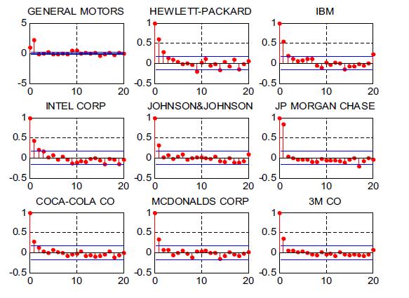
52 3.5 Empirical Results The descriptive statistics is displayed in Table 3.1 for the stock daily returns. The mean of returns across all stocks are no different to zero, however, the standard deviation varies.there is excessive kurtosis for the return series. Figure 3.1 displays the quarterly realized volatility for our 23 DJIA stocks, computed both from 30-minute and daily returns. There is a close correspondence between these two volatility measures, though the volatility measure from daily returns displays some measurement error with an upward bias. Figures 3.6 and 3.6 display the Autocorrelation Functions (ACFs) and Partial Autocorrelation Functions (PACFs) of quarterly logarithmic realized volatility, computed from daily returns, for each stock over the sample period from Q4, 1997 to Q2, The quarterly logarithmic realized volatility have gradual declining autocorrelations for all stocks in our sample and most of the PACFs cut off at lag 1. We next empirically evaluate the three approaches to quarterly volatility forecasting, discussed in the previous section. One quarter ahead forecasts from these models over the forecast evaluation period from Q4, 1997 to Q2, 2008 are measured against the quarterly realized volatility computed from 30-minute returns and overnight returns. The prediction accuracy is evaluated on the basis of mean squared error (MSE) and mean absolute error (MAE) for each stock. The MSE and MAE are computed as follows: MSE = 1 m m ( σ i,r 2 σ i,r 2 )2 (3.9) r=1 MAE = 1 m m σ i,r 2 σ i,r 2 (3.10) r=1 40

53 where σ i,r 2 represents the one-quarter-ahead volatility forecast made at the end of quarter r 1forstocki and σ 2 i,r denotes the realized volatility computed from 30-minute returns and overnight returns in quarter r for stock i. The constant model forecasts are from in-sample estimation periods of 1, 2, 3, 4, 5 and 6 quarters. While the AR model forecasts are from in-sample estimation periods of 20, 30, 40, 50, 60, 70 and 80 quarters. Finally, the MIDAS model forecasts are from an in-sample estimation period of 68 quarters, with MIDAS lag lengths of 40, 60, 80, 100, 150 and 200 trading days. Table 3.2 and 3.3 display the performance of the one-quarter-ahead volatility forecasts. The values of MSE and MAE are the average values over all 23 stocks for each model. The AR(1) model with an in-sample estimation period of 70 quarters produces the lowest MSE and MAE, and , respectively. Not surprisingly given the well known time-variation in volatility, the constant model forecasts perform poorly. Lastly, the MIDAS models demonstrate varying degrees of performance. The unrestricted beta, restricted beta and unrestricted exponential model forecast errors are worse than some of the constant models. Whereas the restricted exponential and hyperbolic model forecast errors are less than the constant models. Relative to the other MIDAS specifications, the hyperbolic model with a lag length of 100 trading days produces the lowest MSE and MAE, and , respectively. Given the lower MSE and MAE results for the AR(1) model, its parsimonious specification and ease of estimation, it dominants the other models for quarterly volatility forecasting. Table 3.4 and 3.5 display the MSE and MAE for the AR(1) one-quarterahead volatility forecast for each stock, with in-sample estimation periods ranging from 20 to 80 quarters. For almost all the stocks, the lowest forecast error is from in-sample 41

54 estimation periods of between 60 and 80 quarters. This suggests that investors with only daily returns can employ the simple AR(1) model with 15 to 20 years historical data to forecast quaterly volatility ahead. 3.6 Conclusions There is a long tradition in the forecasting literature of utilizing parsimonious time series models. Often these models produce the most accurate forecasts. This forecasting principle in the volatility literature was demonstrated by Andersen et al. (2003) where they found standard autoregressive models of daily realized volatility as the dominant forecasting approach for short range volatility, relative to other more complicated commonly used approaches at that time. However, further research by Ghysels et al. (2006) and Corsi (2009) with MIDAS models did find some forecasting improvements over standard autoregressive models of daily realized volatility. In this chapter we find that for longer range volatility forecasts at the quarterly frequency, an autoregressive model with one lag of quarterly realized volatility is the dominant forecasting model. MIDAS models are considered, though they are found to generate inferior forecasts at the quarterly horizon. 42

55 Table 3.1: Descriptive Statistics for stocks and Index Company Name Mean Stdev Min Max Skew Kurtosis AMERICAN EXPRESS AMER INTL GRP INTEL CORP BANK OF AMERICA CORP HOME DEPOT INC MICROSOFT CORP ALCOA INC BOEING CO CATERPILLAR INC JP MORGAN CHASE COCA-COLA CO CITIGROUP INC DISNEY (WALT) CO DU PONT GENERAL ELECTRIC GENERAL MOTORS HEWLETT-PACKARD IBM JOHNSON&JOHNSON MCDONALDS CORP MERCK & CO M CO PFIZER PROCTER & GAMBLE CO A T & T INC UNITED TECH CORP WAL-MART STORES DJIA Index This table presents the descriptive statistics for daily returns of all 23 stocks and Dow Jones Industrial Average Index. We show the mean, standard deviation, minimum, maximum, skew and kurtosis. The data is obtained from the Center for Research in Security Prices (CRSP), with adjustments made for corporate actions, such as dividends, splits etc. Daily return series starts from January 1, 1975 and ends on July 31,

56 Table 3.2: Average MSE of One-Quarter-Ahead Volatility Forecasts A In-Sample Size 1Q 2Q 3Q 4Q 5Q 6Q Constant Model B In-Sample Size 20Q 30Q 40Q 50Q 60Q 70Q 80Q AR(1) AR(2) AR(3) AR(4) AR(5) C MIDAS Specification MIDAS Lag Length BETA BETA REST EXP EXP REST HYPERB For the AR models, the in-sample estimation period is expressed in number of quarters. The constant model forecast is the average of realized volatility over the past quarters. The MIDAS specifications include the unrestricted beta model denoted by BETA, the restricted beta model, denoted by BETA REST, the unrestricted exponential model, denoted by EXP, the restricted exponential model, denoted by EXP REST and the hyperbolic model, denoted by HYPERB. The MIDAS estimation is based on data over the past 68 quarters. The forecast evaluation period is from 1997 Q4 to 2008 Q2. Values are computed by averaging over stocks and the minimum value is highlighted. 44

57 Table 3.3: Average MAE of One-Quarter-Ahead Volatility Forecasts A In-Sample Size 1Q 2Q 3Q 4Q 5Q 6Q Constant Model B In-Sample Size 20Q 30Q 40Q 50Q 60Q 70Q 80Q AR(1) AR(2) AR(3) AR(4) AR(5) C MIDAS Specification MIDAS Lag Length BETA BETA REST EXP EXP REST HYPERB For the AR models, the in-sample estimation period is expressed in number of quarters. The constant model forecast is the average of realized volatility over the past quarters. The MIDAS specifications include the unrestricted beta model denoted by BETA, the restricted beta model, denoted by BETA REST, the unrestricted exponential model, denoted by EXP, the restricted exponential model, denoted by EXP REST and the hyperbolic model, denoted by HYPERB. The MIDAS estimation is based on data over the past 68 quarters. The forecast evaluation period is from 1997 Q4 to 2008 Q2. Values are computed by averaging over stocks and the minimum value is highlighted. 45

58 Table 3.4: MSE of one-quarter-ahead AR(1) volatility forecasts Company In-Sample Size ALCOA INC AMER INTL GRP AMERICAN EXPRESS BOEING CO BANK OF AMERICA CORP CATERPILLAR INC DU PONT DISNEY (WALT) CO GENERAL ELECTRIC GENERAL MOTORS HEWLETT-PACKARD IBM INTEL CORP JOHNSON & JOHNSON JP MORGAN CHASE COCA-COLA CO MCDONALDS CORP M CO MERCK & CO PFIZER PROCTER & GAMBLE CO UNITED TECH CORP WAL-MART STORES The in-sample estimation period is expressed in number of quarters. The forecast evaluation period is from 1997 Q4 to 2008 Q2 and the minimum value is highlighted. 46

59 Table 3.5: MAE of one-quarter-ahead AR(1) volatility forecasts Company In-Sample Size ALCOA INC AMER INTL GRP AMERICAN EXPRESS BOEING CO BANK OF AMERICA CORP CATERPILLAR INC DU PONT DISNEY (WALT) CO GENERAL ELECTRIC GENERAL MOTORS HEWLETT-PACKARD IBM INTEL CORP JOHNSON&JOHNSON JP MORGAN CHASE COCA-COLA CO MCDONALDS CORP M CO MERCK & CO PFIZER PROCTER & GAMBLE CO UNITED TECH CORP WAL-MART STORES The in-sample estimation period is expressed in number of quarters. The forecast evaluation period is from 1997 Q4 to 2008 Q2 and the minimum value is highlighted. 47

60 Figure 3.1: Quarterly Realized Volatility 48

61 49

62 The solid line is the proxy for the true realized volatility which is computed from 30-minute returns and overnight returns. The dotted line is the realized volatility computed from daily returns. The sample covers the period from 1997 Q4 to 2008 Q2, 43 quarters in total. Both volatility measures are multiplied by

63 Figure 3.2: Autocorrelation Functions for Logarithmic Quarterly Realized Volatility 51

64 52

65 The quarterly realized volatility is computed from daily returns and the sample covers the period from 1997 Q4 to 2008 Q2. The marked confidence bands are at the 95% level. 53

66 Figure 3.3: Partial Autocorrelation Functions for Logarithmic Quarterly Realized Volatility 54

67 55