The Pocket CFO: Tools And Metrics

Transcription

1 The Pocket CFO: Tools And Metrics

2 The Pocket CFO: Tools and Metrics Copyright 2014 by DELTACPE LLC All rights reserved. No part of this course may be reproduced in any form or by any means, without permission in writing from the publisher. The author is not engaged by this text or any accompanying lecture or electronic media in the rendering of legal, tax, accounting, or similar professional services. While the legal, tax, and accounting issues discussed in this material have been reviewed with sources believed to be reliable, concepts discussed can be affected by changes in the law or in the interpretation of such laws since this text was printed. For that reason, the accuracy and completeness of this information and the author's opinions based thereon cannot be guaranteed. In addition, state or local tax laws and procedural rules may have a material impact on the general discussion. As a result, the strategies suggested may not be suitable for every individual. Before taking any action, all references and citations should be checked and updated accordingly. This publication is designed to provide accurate and authoritative information in regard to the subject matter covered. It is sold with the understanding that the publisher is not engaged in rendering legal, accounting, or other professional service. If legal advice or other expert advice is required, the services of a competent professional person should be sought. -From a Declaration of Principles jointly adopted by a committee of the American Bar Association and a Committee of Publishers and Associations.

3 Course Description This course is a one-stop problem-solver for today s busy executive. The course is a working guide to help you quickly pinpoint in the complex world of business. What to look for What to do What to watch out for How to do it You ll find ratios, formulas, guidelines, and rules of thumb to help analyze and evaluate any businessrelated problem. Throughout, you ll find this course practical, quick, and useful. Part I takes you through accounting principles and guidelines for evaluating a company s financial health. You will have an increased understanding of various financial statements and their implications. You will be exposed to Corporate Responsibility Law, better known as the Sarbanes-Oxley (SOX) Act. Part II takes a look at financial analysis tools, financial metrics, and financing methods for decision making. Part III takes you through the seemingly complex world of quantitative analysis. You ll use statistics for forecasting and validity testing. Decision theories include linear programming, learning curve theory, and queuing models; these are presented concisely and comprehensively to help you use such sophisticated techniques with relative ease. And, you ll learn how computer applications facilitate the many complex procedures. This course has been designed in question-and-answer format in order to address the pertinent issues that come up during the course of business. Field of Study Level of Knowledge Prerequisite Advanced Preparation Finance Basic to Intermediate None None

4 Table of Contents Chapter 1: Financial Statements, the Sarbanes-Oxley Act, and Corporate Governance... 2 Learning Objectives: What and Why of Financial Statements Classified Financial Statements Statement of Cash Flows Chapter 1 Review Questions Section Cash Flow Analysis Other Sections of the Annual Report Quarterly Report The Management's Discussion and Analysis (MD&A) Section of an Annual Report The Sarbanes-Oxley (Sox) Act Chapter 1 Review Questions Section Chapter 2: How To Evaluate And Improve A Company s Financial Performance Learning Objectives: How To Evaluate A Company s Financial Performance Horizontal and Vertical Analysis Working with Financial Ratios Chapter 2 Review Questions Section How to Analyze and Improve Corporate Profitability and Shareholder Value Return on Investment (ROI) and the Du Pont Formula Return on Equity (ROE) and the Modified Du Pont Formula Chapter 2 Review Questions Section Chapter 3: Internal Accounting Applications for Your Company Learning Objectives: How to Analyze Divisional and Departmental Performance Contribution Margin Analyses Pricing Tools Evaluating the Product Line How to Measure Marketing Effectiveness Chapter 3 Review Questions Section

5 3.6 Budgeting Techniques Highlighting Problem Areas with Variance Analysis Activity-Based Costing (ABC) Life-Cycle Costs and Target Costing Balanced scorecard Chapter 3 Review Questions - Section Chapter 4: Cost-Volume-Profit Analysis, Operating Leverage, and Discounting Analysis Learning Objectives: Cost-Volume-Profit (CVP) Analysis Contribution Margin From Break-Even to Target Profits What-if Analysis Present Proposed Difference Sales Mix Analysis Deluxe Standard Deluxe Standard Budgeted Actual Economy Regular Backpacker Total Operating Leverage Chapter 4 Review Questions Section Time Value of Money Future and Present Values Chapter 4 Review Questions Section Chapter 5: Capital Budgeting

6 Learning Objectives: Capital Budgeting Techniques for Evaluating Investment Proposals Chapter 5 Review Questions Section Effect of Income Taxes on Capital Budgeting Decisions The Lease - Purchase Decision Capital Budgeting and Inflation Chapter 5 Review Questions Section Chapter 6: Assets Management, Financing Techniques, and Portfolio Theory Learning Objectives: Managing Working Capital Maximizing Your Return on Cash Managing Accounts Receivable Formulating the Best Investment Strategy Chapter 6 Review Questions Section How to Best Finance Your Business How to Reduce Risk: Diversify Beta - The Capital Asset Pricing Model (CAPM) The Arbitrage Pricing Model (APM) Chapter 6 Review Questions Section Chapter 7: Decision Making with Statistics and Forecasting Learning Objectives: How to Use Basic Statistics Using Forecasting Techniques Moving Averages Exponential Smoothing Regression Analysis for Sales and Earnings Projections Chapter 7 Review Questions Section What Statistics to Look for in Regression Analysis Statistics to Look For In Multiple Regressions Measuring the Accuracy of Your Forecasts How to Use a Computer Statistical Package for Multiple Regressions Chapter 7 Review Questions Section

7 Chapter 8: Making Use of Quantitative Decision Making Learning Objectives: Decision Making under Risk, Certainty, and Conflict Decision Making Under Uncertain Conditions Decision Theory Linear Programming and Shadow Prices Linear Programming Shadow Prices (Opportunity Costs) How to Use the Computer for Linear Programming Chapter 8 Review Questions Section Learning Curve Inventory Planning and Control Queuing (Waiting Line) Models Chapter 8 Review Questions Section Glossary Index Review Question Answers

8 PREFACE This course is a one-stop problem-solver for today s busy executive. It is a sequel to The Pocket MBA: Concepts and Strategies. The course is a working guide to help you quickly pinpoint in the complex world of business. What to look for What to do What to watch out for How to do it You ll find ratios, formulas, guidelines, and rules of thumb to help you analyze and evaluate any businessrelated problem. Throughout, you ll find this course practical, quick, and useful. Uses for this course are as varied as the topics presented. Part I (Chapters 1, 2, and 3) takes you through accounting principles and guidelines for evaluating a company s financial health. You will have an increased understanding of various financial statements and their implications. You will be exposed to Corporate Responsibility Law, better known as the Sarbanes- Oxley (SOX) Act. You ll learn techniques for analyzing another company s financial position should you wish to invest, extend credit, or compare. You will also learn how to improve a company s corporate profitability and shareholder value. We present internal managerial accounting applications to help you evaluate your own company s performance, profitability, marketing effectiveness, and budgeting process. You ll learn how to highlight problem areas with variance analysis. You will also learn some valuable new tools, such as activity-based costing (ABC), life-cycle costing, target costing, and corporate balanced scorecard. Part II (Chapters 4, 5, and 6) takes a look at financial analysis tools, financial metrics, and financing methods for decision making. Through break-even and sensitivity analysis, you ll be able to move your company toward greater profits. For investment purposes, this part presents guidelines for evaluating proposals, whether they be short or long term, for profit potential and risk-return comparisons. You ll learn management and financing techniques to ensure the best possible strategies for maximizing and acquiring cash. Also covered are basic financial tenets of portfolio theory, the Capital Asset Pricing Model (CAPM), and the Arbitrage Pricing Model (APM). Part III (Chapters 7 and 8) takes you through the seemingly complex world of quantitative analysis. You ll use statistics for forecasting and validity testing. Decision theories include linear programming, learning curve theory, and queuing models; these are presented concisely and comprehensively to help you use such sophisticated techniques with relative ease. And, you ll learn how computer applications facilitate the many complex procedures. Computer applications are heavily stressed throughout the chapters. This course has been designed in question-and-answer format in order to address the pertinent issues that come up during the course of business. The questions are typical of those asked by persons like yourself. The answers are clear, concise, and to the point. In short, this is a veritable cookbook of guidelines, illustrations, and how-to s for you, the modern decision maker. 1

9 Chapter 1: Financial Statements, the Sarbanes-Oxley Act, and Corporate Governance Learning Objectives: After completing this section, you should be able to: Understand the objectives of financial reporting and the key elements contained within different financial statements. Recognize the purpose and content of the statement of cash flows. Identify key sections contained with the annual report. Recognize issues addressed by the Sarbanes-Oxley (SOX) Act and the groups impacted by it. Knowing the financial health of your company is important. Such knowledge can help you allocate resources and pinpoint areas requiring development and problems needing correction. Do you know how your company is doing financially? Is it growing or contracting? Will it be around for a long time? How profitable is your department, and what can be done to improve the profitability picture? These questions and others can be answered if you understand corporate financial statements. On the other hand, if you do not know how your company is doing financially, you cannot provide the needed financial leadership. A series of accounting scandals on the heels of the infamous Enron debacle, coupled with frequent financial restatements because of financial reporting fraud and/or accounting errors, have led to new sweeping accounting guidelines, proposals, and legislation, notably the Sarbanes-Oxley (SOX) Act in 2002 This chapter looks at the key financial statements from an external viewpoint. The Sarbanes-Oxley (SOX) Act is also summarized. 2

10 1.1 What and Why of Financial Statements What are financial statements? What is their significance? Financial decisions are typically based on information generated from the accounting system. Financial management, stockholders, potential investors, and creditors are concerned with how well the company is doing. The three reports generated by the accounting system and included in the company's annual report are the balance sheet, income statement, and statement of cash flows. Although the form of these financial statements may vary among different businesses or other economic units, their basic purposes do not change. The objectives of financial reporting are concerned with the underlying goals and purposes of accounting. They are to provide information that (1) is useful to those making investment and credit decisions, assuming that those individuals have a reasonable understanding of business and economic activities; (2) is helpful to current and potential investors and creditors and other users such as labor and government agencies in assessing the amount, timing, and uncertainty of future cash flows; and (3) discloses economic resources, claims to those resources, and the changes therein. The balance sheet portrays the financial position of the organization at a particular point in time. It shows what you own (assets), how much you owe to vendors and lenders (liabilities), and what is left (assets minus liabilities, known as equity or net worth). A balance sheet is a snapshot of the company's financial position as of a certain date. The balance sheet equation can be stated as: Assets - Liabilities = Stockholders' Equity. The income statement, on the other hand, measures the operating performance for a specified period of time (e.g., for the year ended December 31, 2X12). If the balance sheet is a snapshot, the income statement is a motion picture. The income statement serves as the bridge between two consecutive balance sheets. Simply put, the balance sheet indicates the wealth of your company and the income statement tells you how your company did last year. The balance sheet and the income statement tell different things about your company. For example, the fact the company made a big profit last year does not necessarily mean it is liquid (has the ability to pay current liabilities using current assets) or solvent (noncurrent assets are enough to meet noncurrent liabilities). A company may have reported a significant net income but still have a deficient net worth. In other words, to find out how your organization is doing, you need both statements. The income statement summarizes your company's operating results for the accounting period; these results are reflected in the equity (net worth) on the balance sheet. This relationship is shown in Figure 1.1. The third basic financial statement is the statement of cash flows. This statement provides useful information about the inflows and outflows of cash that cannot be found in the balance sheet and the income statement. 3

11 Figure 1.1 The Balance Sheet and Income Statement Figure 1.2 shows how these statements, including the statement of retained earnings (to be discussed later), tie together with numerical figures. NOTE: The beginning amount of cash ($50 million) from the 2X12 balance sheet is added to the net increase or decrease in cash (from the statement of cash flows) to derive the cash balance ($111 million) as reported on the 2X12 balance sheet. Similarly, the retained earnings balance as reported on the 2X12 balance sheet comes from the beginning retained earnings balance (2X12 balance sheet) plus net income for the period (from the income statement) less dividends paid. As you study financial statements, these relationships will become clearer and you will understand the concept of articulation better. 4

12 Figure 1.2 How the Financial Statements Tie Together Statement of Cash Flows 12/31/2x11-12/31/2x12 (in millions) Operating activities $ 1,488.4 Investing activities (2,064.3) Financing activities Net increase in cash $ 60.5 Beginning cash 50.0 Ending cash $ Balance Sheet, 12/31/2x11 Balance Sheet, 12/31/2x12 Cash $ 50.0 Income Statement, 12/31/2x11-12/31/2x12 Cash $ All other assets 11,339.6 Revenues $ 28,898.2 All other assets 14,794.1 $ 11,389.6 Expenses 27,927.3 $ Liabilities $ 8,307.5 Liabilities $ 10,814.5 Capital stock 1,157.1 Net income $ Capital stock 1,194.2 Retained earnings 1,925.0 Retained earnings 2,895.9 $ 11,389.6 $ 14,904.6 Statement of Retained Earnings 12/31/2x11-12/31/2x12 Retained earnings, 12/31/2x11 $ 1,925.0 Net income Dividends 0 Retained earnings, 12/31/2x12 $ 2,895.9 What does the income statement tell you? The income statement (profit and loss statement) shows the revenue, expenses, and net income (or net loss) for a period of time. It is typically dated For the year ended December 31, 2XXX. A definition of each element follows. Revenue is the increase in capital arising from the sale of merchandise or the performance of services. When revenue is earned, it results in an increase in either cash (money received) or accounts receivable (amounts owed to you by customers). Expenses decrease capital and result from performing activities necessary to generate revenue. Expenses that reduce net income can be categorized as the cost of goods sold and selling and general administrative expenditures necessary to conduct business operations (e.g., rent expense, salary expense, depreciation expense) during the period. Net income is the amount by which total revenue exceeds total expenses. The resulting profit is added to the retained earnings account (accumulated earnings of a company since its inception less dividends). If total expenses are greater than total revenue, a net loss results, decreasing retained earnings. Revenue does not necessarily mean receipt of cash, and expense does not automatically imply a cash payment. Net income and net cash flow (cash receipts less cash payments) are different. For example, taking out a bank loan generates cash, but this cash is not revenue since no merchandise has been sold and 5

13 no services have been provided. Further, owners equity does not change as the loan represents a liability, rather than a stockholders' investment, and must be repaid. Each revenue and expense item has its own account. Such a system enables you to better evaluate and control revenue and expense sources and to examine the relationships among account categories. 1.2 Classified Financial Statements Although companies differ in nature and therefore the specific transactions and accounts differ from business to business, it is useful to classify the entries in financial statements into major categories. Financial statements organized in such a fashion are called classified financial statements. How detailed is a classified income statement? In a classified income statement, each major revenue and expense function is listed separately to facilitate analysis. The entries in an income statement are usually classified into four major functions: revenue, cost of goods sold (cost of inventory sold), operating expenses, and other revenue or expenses. The entries in classified income statements covering different time periods are easily compared; the comparison over time of revenue sources, expense items, and the relationship between them can reveal areas that require attention and corrective action. For example, if revenue from services has been sharply declining over the past several months, you will want to know why and then take action to reverse the trend. Revenue comprises the gross income generated by selling goods (sales) or performing services (professional fees, commission income). To determine net sales, gross sales are reduced by sales returns, allowances (discounts given for defective merchandise), and sales discounts. Cost of goods sold is the cost of the merchandise or services sold. In a retail business, the cost of goods sold is the beginning inventory plus the cost of buying goods from the manufacturer minus ending inventory; in a service business, it is the cost of the employee services rendered. For a manufacturing company, cost of goods sold is the cost of goods manufactured plus the beginning finished goods inventory minus the ending finished goods inventory. Operating expenses are expenses incurred or resources used in generating revenue. Two types of operating expenses are selling expenses and general and administrative expenses. Selling expenses are costs incurred in the sale of goods or services (e.g., advertising, salesperson salaries) and in distributing the merchandise (e.g., freight paid on shipments); they relate solely to the selling function. If a sales manager is responsible for generating sales, his or her performance is judged on the relationship between promotion costs and sales obtained. General and administrative expenses are the costs of running the business as a whole. The salaries of the office clerical staff, administrative executive salaries, and depreciation on office equipment are examples of general and administrative expenses. 6

14 Other revenue (expenses) covers incidental sources of revenue and expense that are nonoperating in nature and that do not relate to the major purpose of the business. Examples are interest income, dividend income, and interest expense. Figure 1.3 shows a classified income statement. FIGURE 1.3 A CLASSIFIED INCOME STATEMENT - X COMPANY For the Year Ended December 2X12 7

15 What is a classified balance sheet? The balance sheet is classified into major groups of assets, liabilities, and owners' equity. An asset is something owned, such as land and automobile; a liability is something owed, such as loans payable and mortgage payable. Owners' equity is the residual interest remaining after assets have been reduced by liabilities. Assets A classified balance sheet generally breaks down assets into five categories: current assets, long-term investments, property, plant, and equipment (fixed assets), intangible assets, and deferred charges. This breakdown aids in analyzing the type and liquidity of the assets held. Current assets are assets expected to be converted into cash or used up within one year or the normal operating cycle of the business, whichever is greater. (The operating cycle is the time period between the purchase of inventory merchandise for resale and the transfer of inventory through sales, listed as accounts receivable, or receipt of cash. In effect, the operating cycle takes you from paying cash to receiving it.) Examples of current assets are cash, short-term investments or short-term investments (investments with a maturity of more than 90 days but intended to be held only until cash is needed for current operations), accounts receivable, inventory, and prepaid expenses (expenditures that will expire within one year from the balance sheet date and that represent a prepayment for an expense that has not yet been incurred.) Long-term investments refer to investments in other companies' stocks (common or preferred) or bonds where the intent is to hold them for a period greater than one year. Securities that may be held as shortterm or long-term investments fall into three categories: held-to-maturity securities, trading securities, and available-for-sale securities. Trading securities are classified as short-term investments. Available-for-sale securities, depending on the company s intent to hold them, may be classified as either short-term or longterm investments. However, in almost all cases, they are noncurrent. Held-to-maturity securities are always classified as long-term investment. Property, plant, and equipment (often called fixed assets) are assets employed in the production of goods or services that have a life greater than one year. They are tangible, meaning they have physical substance (you can physically see and touch them) and are actually being used in the course of business. Examples are land, buildings, machinery, and automobiles. Unlike inventory, these assets are not held for sale in the normal course of business. Intangible assets are assets with a long-term life that lack physical substance and that arise from a right granted by the government, such as patents, copyrights, and trademarks, or by another company, such as a franchise license. An example of the latter is the right (acquired by paying a fee) to open a fast food franchise and use the name of McDonald's. Deferred charges are certain expenditures that have already been incurred but that are deferred to the future either because they are expected to benefit future revenues or because they represent an appropriate allocation of costs to future operations. In other words, deferred charges are costs charged to 8

16 an asset because future benefit exists; they are amortized as an expense in the year the related revenue is recognized and the benefit consumed in conformity with the accounting principle requiring matching of expense to revenue. Examples are plant rearrangement costs and moving costs. No cash can be realized from such assets; for example, you cannot sell deferred moving costs to anyone because no one will buy them. Liabilities and Stockholders' Equity Liabilities are classified as either current or noncurrent. Current liabilities (those due in one year or less) will be satisfied out of current assets. Examples are accounts payable (amounts owed to creditors), short-term notes payable (written evidence of loans due within one year), and accrued expense liabilities (e.g., salaries payable). Examples of long-term liabilities, which have a maturity of greater than one year, are bonds payable and mortgage payable. The current portion of a long-term liability (that part that is to be paid within one year) is shown under current liabilities. For example, if $1,000 of a $10,000 mortgage is to be paid within the year, that $1,000 is listed as a current liability; the remaining $9,000 is shown under noncurrent liabilities. The stockholders' equity section of the balance sheet consists of capital stock, paid-in-capital, retained earnings, and total stockholders' equity. These are defined below. Capital stock describes the ownership of the corporation in terms of the number of shares outstanding. Each share is assigned a par value when it is first authorized by the state in which the business is incorporated. Capital stock is presented on the balance sheet at total par value. Therefore, the capital stock account, which is at par value, agrees with the stock certificates (imprinted with the par value) held by stockholders. Preferred stock is listed before common stock because it receives preference should the company be liquidated. Paid-in capital shows the amount received by the company over the par value for the stock issued. This helps keep track of the par value of issued shares and the excess over par value paid for it. Retained earnings represent the accumulated earnings of the company since its inception less dividends declared and paid to stockholders. There is usually a surplus in this account, but a deficit may occur if the business has been operating at a loss. Total stockholders' equity is the sum of capital stock, paid-in capital, and retained earnings. In a corporation, owners' equity is referred to as stockholders' equity; in a sole proprietorship or partnership, owners' equity is referred to as capital. A classified balance sheet is presented in Figure

17 FIGURE 1.4 BALANCE SHEET - X COMPANY DECEMBER 31, 2X12 10

18 1.3 Statement of Cash Flows Why is the statement of cash flows so important? It is important to know your cash flow so that you may adequately plan your expenditures. Should there be a cut back on payments because of a cash problem? Is the organization getting most of your cash? What products or projects are cash drains or cash cows? Is there enough money to pay bills and buy needed machinery? A Statement of Cash Flows is required to be prepared by all business enterprises and nonprofit organizations. It contains useful information for external users, such as lenders and investors, who make economic decisions about a company. The statement presents the sources and uses of cash and is a basis for cash flow analysis. In this section, we discuss what the statement of cash flows is, how it looks, and how to analyze it. What are the specific contents of the statement of cash flows? The statement of cash flows classifies cash receipts and cash payments arising from investing activities, financing activities, and operating activities. Investing Activities Investing activities include the results of the purchase or sale of debt and equity securities of other entities and fixed assets. Cash inflows from investing activities are comprised of (1) receipts from sales of equity and debt securities of other companies and (2) amounts received from the sale of fixed assets. Cash outflows for investing activities include (1) payments to buy equity or debt securities of other companies and (2) payments to buy fixed assets. Financing Activities Financing activities include the issuance of stock and the reacquisition of previously issued shares (treasury stock), as well as the payment of dividends to stockholders. Also included are debt financing and repayment. Cash inflows from financing activities are comprised of funds received from the sale of stock and the incurrence of debt. Cash outflows for financing activities include (1) repaying debt, (2) repurchasing of stock, and (3) issuing dividend payments. Operating Activities Operating activities are connected to the manufacture and sale of goods or the rendering of services. Cash inflows from operating activities include (1) cash sales or collections on receivable arising from the initial sale of merchandise or rendering of service and (2) cash receipts from debt securities (e.g., interest income) 11

19 or equity securities (e.g., dividend income) of other entities. Cash outflows for operating activities include (1) cash paid for raw material or merchandise intended for resale, (2) payments on accounts payable arising from the initial purchase of goods, (3) payments to suppliers of operating expense items (e.g., office supplies, advertising, insurance), and (4) wages. Figure 1.5 shows an outline of the statement of cash flows. FIGURE 1.5 THE STATEMENT OF CASH FLOWS 12

20 Chapter 1 Review Questions Section 1 1. Financial decisions are typically based on three reports: Gant Load Chart, Gant scheduling chart, and the Program Evaluation and Review Technique (PERT). True or False? 2. An objective of financial reporting is A. Providing information useful to investors, creditors, management, labor, and government agencies, and other users for decision making. B. Assessing the adequacy of internal control. C. Evaluating management results compared with standards. D. Providing information on compliance with established procedures. 3. The primary purpose of the balance sheet is to reflect A. The fair value of the firm s assets at some moment in time. B. The status of the firm s assets in case of forced liquidation of the firm. C. Assets, liabilities, and equity. D. The firm s potential for growth in stock values in the stock market. 4. Revenue always means receipt of cash, and expenses automatically implies cash payment. True or False? 5. Intangible assets are often called fixed assets that are employed in the production of goods and/or services that have a life greater than one year. True or False? 6. The amount received by a company over par value for stock is paid-in capital. True or False? 7. The statement of cash flows is required in annual reports since it is for external use only. True or False? 8. A financial statement includes all of the following items: operating activities, financial activities and investing activities. What financial statement is this? 13

21 A. Statement of cash flows. B. Balance sheet. C. Income statement. D. Statement of retained earnings. 14

22 1.4 Cash Flow Analysis How do you analyze the cash flow position of a company? Along with financial ratio analysis, cash flow analysis is a valuable tool. The cash flow statement provides information on how your company generated and used cash, that is, why cash flow increased or decreased. An analysis of the statement is helpful in appraising past performance, projecting the company's future direction, forecasting liquidity trends, and evaluating your company's ability to satisfy its debts at maturity. CHECKLIST FOR CASH FLOW ANALYSIS QUESTIONS Because the statement lists the specific sources and uses of cash during the period, it can be used to answer the following: How was the expansion in plant and equipment financed? What use was made of net income? Where did you obtain funds? How much required capital is generated internally? Is the dividend policy in balance with its operating policy? How much debt was paid off? How much was received from the issuance of stock? How much debt financing was taken out? The cash flow per share equals net cash flow divided by the number of shares. A high ratio is desirable because it indicates a liquid position, that is, that the company has ample cash on hand. Operating Section An analysis of the operating section of the statement of cash flows determines the adequacy of cash flow from operating activities. For example, an operating cash outlay for refunds given to customers for deficient goods indicates a quality problem with the merchandise, while payments of penalties, fines, and lawsuit damages reveal poor management practices that result in non-beneficial expenditures. Investing Section An analysis of the investing section can identify investments in other companies. These investments may lead to an attempt to assume control of another company for purposes of diversification. The analysis may also indicate a change in future direction or a change in business philosophy. 15

23 An increase in fixed assets indicates capital expansion and future growth. A contraction in business arising from the sale of fixed assets without adequate replacement is a negative sign. Financing Section An evaluation of the financing section reveals the company's ability to obtain financing in the money and capital markets as well as its ability to meet obligations. The financial mixture of bonds, long-term loans from banks, and equity instruments affects risk and the cost of financing. Debt financing carries greater risk because the company must generate adequate funds to pay the interest costs and to retire the obligation at maturity; thus, a very high percent of debt to equity is generally not advisable. The problem is acute if earnings and cash flow are declining. On the other hand, reducing long-term debt is desirable because it points to lowered risk. The ability to obtain financing through the issuance of common stock at attractive terms (high stock price) indicates that the investing public is optimistic about the financial well-being of the business. The issuance of preferred stock may be a negative sign, since it may mean the company is having difficulty selling its common stock. Perhaps investors view the company as very risky and will invest only in preferred stock since preferred stock has a preference over common stock in the event of the company's liquidation. Evaluate the company's ability to pay dividends. Stockholders who rely on a fixed income, such as a retired couple, may be unhappy when dividends are cut or eliminated. 16

24 How do you prepare and analyze the statement of cash flows? In this section, we do an analysis of a hypothetical statement of cash flows, prepared from sample balance sheet and income statement figures. EXAMPLE 1.1 X Company provides the following financial statements: 17

25 Assume the company has a policy of paying very high dividends. Information for 2X11 follows: Net income, $32; cash flow from operations, $20. A financial analysis of the statement of cash flows reveals that the profitability and operating cash flow of X Company improved from 2X11 to 2X12. The company's earnings performance was good, and the $61 earnings resulted in cash inflow from operations of $75. Thus, compared to 2X11, 2X12 showed better results. The decrease in accounts receivable may reveal better collection efforts. The increase in accounts payable is a sign that suppliers are confident they will be paid and are willing to give interest-free financing. The acquisition of land, building, and equipment points to a growing business undertaking capital expansion. The issuance of long-term notes payable indicates that the company is financing part of its assets through debt. Stockholders will be happy with the significant dividend payout of 80.3 percent (dividends divided by net income, or $49/$61). Overall, there was a decrease in cash on hand of $7, but this should not cause alarm because of the company's profitability and the fact that cash was used for capital expansion and dividend payments. We recommend that the dividend payout be reduced from its high level and that the funds be reinvested in the business; the reduction of dividends by more than $7 would result in a positive net cash flow for the year, which is needed for immediate liquidity. 18

26 EXAMPLE 1.2 Y Company presents the following statement of cash flows. An analysis of the statement of cash flows reveals that the company is profitable and that cash flow from operating activities exceeds net income, which indicates good internal cash generation. The ratio of cash flow from operating activities to net income is a solid 1.45 ($194,000/$134,000). A high ratio is desirable because it shows that earnings are backed up by cash. The decline in accounts receivable may indicate better collection efforts; the increase in accounts payable shows the company can obtain interest-free financing. The company is definitely in the process of expanding for future growth, as demonstrated by the purchase of land, building, and equipment. The debt position of the company has increased, indicating greater risk for investors. The dividend payout was 13.4 percent ($18,000/$134,000), which is good news for stockholders, who look positively on companies that pay dividends. The decrease of $12,000 in cash flow for the year is a negative sign. How can you use the statement of cash flows for corporate planning? Current profitability is only one important factor in predicting corporate success; current and future cash flows are also essential. In fact, it is possible for a profitable company to have a cash crisis; for example, a company with significant credit sales but a very long collection period may show a profit without actually having the cash from those sales. 19

27 Financial managers are responsible for planning how and when cash will be used and obtained. When planned expenditures require more cash than planned activities are likely to produce, financial managers must decide what to do. They may decide to obtain debt or equity funds or to dispose of some fixed assets or a whole business segment. Alternatively, they may decide to cut back on planned activities by modifying operational plans, such as ending a special advertising campaign or delaying new acquisitions, or to revise planned payments to financing sources, such as bondholders or stockholders. Whatever is decided, the financial manager's goal is to balance the cash available and the needs for cash over both the short and the long term. Evaluating the statement of cash flows is essential if you are to appraise accurately an entity's cash flows from operating, investing, and financing activities and its liquidity and solvency positions. Inadequacy in cash flow has possible serious implications, including declining profitability, greater financial risk, and even possible bankruptcy. 1.5 Other Sections of the Annual Report What other crucial information the annual report contains? Other sections in the annual report in addition to the financial statements are helpful in understanding the company's financial health. These sections include the highlights, review of operations, footnotes, supplementary schedules, and auditor's report. Highlights The highlights section provides comparative financial statement information and covers important points such as profitability, sales, dividends, market price of stock, and asset acquisitions. At a minimum, the company provides sales, net income, and earnings per share figures for the last two years. Review of Operations The review of operations section discusses the company's products, services, facilities, and future directions in both numbers and narrative form. Report of Independent Public Accountants The independent accountant is a certified public accountant (CPA) in public practice who has no financial or other interest in the client whose financial statements are being examined. In this part of the annual report, he or she expresses an opinion on the fairness of the financial statement numbers. 20

28 CPAs render four types of audit opinions: an unqualified opinion, a qualified opinion, a disclaimer of opinion, and an adverse opinion. The auditor's opinion is heavily relied on since he or she is knowledgeable, objective, and independent. Unqualified Opinion. An unqualified opinion means the CPA is satisfied that the company's financial statements present fairly its financial position and results of operations and gives the financial manager confidence that the financial statements are an accurate reflection of the company's financial health and operating performance. A typical standard report presenting an unqualified opinion follows. Independent Auditor's Report We have audited the accompanying balance sheet of ABC Company as of December 31, 2X12 and the related statements of income, retained earnings, and cash flows for the year then ended. These financial statements are the responsibility of the Company's management. Our responsibility is to express an opinion on these financial statements based on our audit. We conducted our audit in accordance with generally accepted auditing standards in the Unites States. Those standards require that we plan and perform the audit to obtain reasonable assurance about whether the financial statements are free of material misstatement. An audit includes examining, on a test basis, evidence supporting the amounts and disclosures in the financial statements. An audit also includes assessing the accounting principles used and significant estimates made by management, as well as evaluating the overall financial statement presentation. We believe that our audit provides a reasonable basis for our opinion. In our opinion, the financial statements referred to above present fairly, in all material respects, the financial position of ABC Company as of December 31, 2X12, and the results of its operations and its cash flows for the year then ended in conformity with generally accepted accounting principles (GAAP). Note: GAAP are the "conventions, rules, and procedures necessary to define accepted accounting at a particular time." They include both the broad guidelines and the detailed practices and procedures promulgated by the profession that provide uniform standards to measure financial presentations. If the company is facing a situation with an uncertain outcome that may substantially affect its financial health, such as a lawsuit, the CPA may still give an unqualified opinion. However, there will probably be an explanatory paragraph describing the material uncertainty; this uncertainty will undoubtedly affect readers' opinions of the financial statement information. As a financial manager, you are well advised to note the contingency (potential problem, such as a dispute with the government) and its possible adverse financial effects on the company. 21

29 Qualified Opinion. The CPA may issue a qualified opinion if your company has placed a "scope limitation" on his or her work. A scope limitation prevents the independent auditor from doing one or more of the following: (1) gathering enough evidential matter to permit the expression of an unqualified opinion; (2) applying a required auditing procedure; or (3) applying one or more auditing procedures considered necessary under the circumstances. If the scope limitation is fairly minor, the CPA may issue an "except for" qualified opinion. This may occur, for example, if the auditor is unable to confirm accounts receivable or observe inventory. Disclaimer of Opinion. When a severe scope limitation exists, the auditor may decide to offer a disclaimer of opinion. A disclaimer indicates that the auditor was unable to form an opinion on the fairness of the financial statements. Adverse Opinion. The auditor may issue an adverse opinion when the financial statements do not present the company's financial position, results of operations, retained earnings, and cash flows fairly and in conformity with GAAP. By issuing an adverse opinion, the CPA is stating that the financial statements may be misleading. Obviously, the financial manager wants the independent auditor to render an unqualified opinion. Disclaimers and adverse opinions are viewed very negatively by readers such as investors and creditors, who then put little if any faith in the company's financial statements. Notes Financial statements themselves are concise and condensed, and any explanatory information that cannot readily be abbreviated is added in greater detail in the notes. In such cases, the report contains a statement similar to this: "The accompanying notes are an integral part of the financial statements." Notes provide detailed information on financial statement figures, accounting policies, explanatory data such as mergers and stock options, and any additional disclosure. Notes disclosures usually include accounting methods, estimated figures such as inventory pricing, pension fund, and profit-sharing arrangements, terms and characteristics of long-term debt, particulars of lease agreements, contingencies, and tax matters. The notes appear at the end of the financial statements and explain the figures in those statements both in narrative form and in numbers. It is essential that the financial manager evaluate notes information to arrive at an informed opinion about the company's financial stature and earning potential. Supplementary Schedules and Tables Supplementary schedules and tables enhance the financial manager's comprehension of the company's financial position. Some of the more common schedules are five-year summary of operations, two-year quarterly data, and segmental information. This summary provides income statement information for the 22

30 past five years, including dividends on preferred stock and common stock. It also reveals operating trends. Some companies provide ten-year comparative data. Two-Year Quarterly Data. This schedule gives a quarterly breakdown of sales, profit, high and low stock price, and the common stock dividend. Quarterly operating information is particularly useful for a seasonal business, because it helps readers to track the business's highs and lows more accurately. The quarterly market price reveals fluctuations in the market price of stock, while the dividend quarterly information reveals how regularly the company pays dividends. Segmental Disclosure. This important supplementary schedule presents financial figures for the segments of the business, enabling readers to evaluate each segment's profit potential and risk. Segmental data may be organized by industry, foreign area, major customer, or government contract. A segment is reportable if any one of the following conditions exists: Revenue is 10 percent or more of total corporate revenue. Operating profit is 10 percent or more of total corporate operating profit. Identifiable assets are 10 percent or more of total corporate assets. The company must also disclose if foreign operations, sales to a major customer, or domestic contract revenue provide 10 percent or more of total sales. The percentage derived and the source of the sales must be stated. Useful segment information that may be disclosed includes sales, operating profit, total assets, fixed assets, intangible assets, inventory, cost of sales, depreciation, and amortization. History of Market Price While this information is optional, many companies provide a brief history of the market price of stock, such as quarterly highs and lows. This information reveals the variability and direction in market price of stock. 1.6 Quarterly Report How do you read a quarterly report? In addition to the annual report, publicly-held companies issue quarterly reports that provide updated information on sales and earnings and describe any material changes that have occurred in the business or its operations. These quarterly reports may provide unaudited financial statements or updates on 23

31 operating highlights, changes in outstanding shares, compliance with debt restrictions, and pending lawsuits. At a minimum, quarterly reports must provide data on sales, net income, taxes, nonrecurring revenue and expenses, accounting changes, contingencies (e.g., tax disputes), additions or deletions of business segments, and material changes in financial position. The company may provide financial figures for the quarter itself (e.g., the third quarter, from July 1 to September 30) or cumulatively from the beginning of the year (cumulative up to the third quarter, or January 1 to September 30). Prior-year data must be provided in a form that allows for comparisons. The financial manager should read the quarterly report in conjunction with the annual report. 1.7 The Management's Discussion and Analysis (MD&A) Section of an Annual Report What does the management's discussion and analysis (MD&A) section of an annual report address to the user? The Management's Discussion and Analysis (MD&A) section of an annual report must be included in SEC filings. The content of the MD&A section is required by regulations of the SEC. The MD&A contains standard financial statements and summarized financial data for at least 5 years. Other matters must be included in annual reports to shareholders and in Form 10-K filed with the SEC. It addresses in a nonquanitified manner the prospects of the company. The SEC examines it with care to determine that management has disclosed material information affecting the company's future results. Disclosures about commitments and events that may affect operations or liquidity are mandatory. Thus, the MD&A section pertains to liquidity, capital resources, and results of operations. 1.8 The Sarbanes-Oxley (Sox) Act What sweeping changes the Sarbanes-Oxley (sox) act involve in corporate financial reporting? President George W. Bush signed the Sarbanes-Oxley Act of 2002 (Public Law ) on Tuesday, July 30, Congress presented the Act ( to the president on July 26, 2002, after passage in the Senate by a 99-0 vote and in the House by a margin. GROUPS IMPACTED BY THE ACT 1. CPAs and CPA firms auditing public companies; 24

32 2. Publicly traded companies, their employees, officers, and owners including holders of more than 10 percent of the outstanding common shares. This category would include CPAs employed by publicly traded companies as chief financial officers (CFOs) or in the finance department; 3. Attorneys who work for or have as clients publicly traded companies; and 4. Brokers, dealers, investment bankers and financial analysts who work for these companies. The Act changes how publicly traded companies are audited, and reshapes the financial reporting system. This Act adopts tough new provisions to deter and punish corporate and accounting fraud and corruption, ensures justice for wrongdoers, and protects the interests of workers and shareholders. This bill improves the quality and transparency of financial reporting, independent audits, and accounting services for public companies. It also: Creates a Public Company Accounting Oversight Board ( to enforce professional standards, ethics, and competence for the accounting profession; Strengthens the independence of firms that audit public companies; Increases corporate responsibility and the usefulness of corporate financial disclosure; Increases penalties for corporate wrongdoing; Protects the objectivity and independence of securities analysts; and Increases Securities and Exchange Commission resources. REMEMBER THIS: Under this law, CEOs and CFOs must personally vouch for the truth and fairness of their company's disclosures. And those financial disclosures will be broader and better than ever before. Corporate officials will play by the same rules as their employees. In the periods when workers are prevented from buying and selling company stock in their pensions or 401 (k)s, corporate officials will also be banned from any buying or selling. Corporate misdeeds will be found and punished. This law authorizes new funding for investigators and technology at the SEC to uncover wrongdoing. The SEC will now have the administrative authority to bar dishonest directors and officers from ever again serving in positions of corporate responsibility. The penalties for obstructing justice and shredding documents are greatly increased. Specifics New Public Company Accounting Oversight Board (PCAOB) The law establishes a five-member Public Accounting Oversight Board (PCAOB) that is subject to Securities and Exchange Commission (SEC) oversight. Though the board oversees accounting firms, only two members of the board may be CPAs. 25

33 The SEC will appoint the board. Duties of the board include registering public accounting firms that prepare audit reports; and establishing or adopting auditing, quality control, ethics and independence standards. The board also inspects, investigates and disciplines public accounting firms and enforces compliance with the act. Registration with the Board Is Mandatory. For public accounting firms, foreign or domestic, that participates in the preparation or issuance of any audit report with respect to a public company. Registration and annual fees collected from each registered CPA firm will go towards the costs of processing and reviewing applications and annual reports. Seven-Year Record Retention Requirement. PCAOB must adopt a rule to require registered CPA firms to prepare and maintain audit work papers and other information related to an audit for at least seven years in sufficient detail to support the conclusions reached in the audit report. (A separate criminal provision requires retention of all audit and review workpapers for five years from the end of the fiscal year in which the audit or review was completed.) Cooperation with CPA Groups. The board will cooperate with professional accountant groups and advisory groups to increase the effectiveness of the standards setting process. (The PCAOB may cooperate, but authority to set standards rests with the PCAOB, subject to SEC review.) Annual Inspections. Inspection of registered public accounting firms shall occur annually for every registered public accounting firm that regularly provides audit reports for more than 100 issuers (at least once every three years for registered firms that audit fewer than 100 issuers). Investigations. The board may investigate any act, omission or practice by a registered firm or an individual associated with a registered firm for any possible violation of the act, the board s rules, professional standards, or provisions of the securities laws relating to the preparation and issuance of audit reports. o The board may require testimony or documents and information (including audit work papers) from a registered firm or individual associated with a registered firm or in the possession of any other person. Sanctions for violations that the board finds may include: o Suspension or revocation of a registration; o Suspension or bar of a person from further associating with any registered public accounting firm; o Limitations on the activities of a firm or person associated with the firm; and o Penalize the firm up to $2 million per violation, up to a maximum of $15 million. o Individuals employed or associated with a registered firm who violate the act can face penalties that range from required additional continuing professional education (CPE) or training, disbarment of the individual from further association with any registered public accounting firm, or even a fine up to $100,000 for each violation, up to a maximum of $750,000. A portion of the penalties collected will go to accounting scholarships. Funding. The law also provides independent funding for the Financial Accounting Standards Board (FASB). While the SEC and American Institute of CPAs (AICPA) both have recognized FASB as the standard setting body for accounting principles, federal authority to issue auditing, quality control, 26

34 ethics and independence standards may seriously impact the AICPAs role in official pronouncements. (a) Source. The budget for the board and FASB will be payable from annual accounting support fees set by the board and approved by the Commission. The fees will be collected from publicly traded companies and will be determined by dividing the average monthly equity market capitalization of the company for the preceding fiscal year by the average monthly equity market capitalization of all such companies for that year. Other Requirements for CPA Firms Most Consulting Banned for Audit Clients. Title II of the act prohibits most consulting services outside the scope of practice of auditors. Services are prohibited even if pre-approved by the issuer s audit committee. o Prohibited services include: Bookkeeping and related services, Design and implementation of financial information systems, Appraisal or valuation services (including fairness opinions and contribution-in-kind reports), Actuarial services, Internal audit outsourcing, Services that provide any management or human resources, Investment or broker/dealer services, and Legal and expert services unrelated to the audit. Any other service that the board determines, by regulation, is impermissible. o Services Not Prohibited. Firms, however, may provide tax services (including tax planning and tax compliance) or others that are not listed, provided the firm receives pre-approval from the board. However, certain tax planning products, like tax avoidance services, may be considered prohibited nonaudit services. Audit Reports Require Concurring Partner Review. Requires a concurring or second partner s review and approval of all audit reports and their issuance. Revolving Door Employment of CPAs with Audit Clients Is Banned. A registered CPA firm is prohibited from auditing any SEC registered client whose chief executive, CFO, controller or equivalent was on the audit team of the firm within the past year. Audit Partner Rotation Required. Audit partners who either have performed audit services or been responsible for reviewing the audit of a particular client must be rotated every five consecutive years. CPAs should read carefully the requirements for rotation of both the partner-in-charge and the concurring review partner for certain organizational constraints. o No Firm Rotation Requirement. Firm rotation is not required. CPA Firms Are Required to Report Directly to the Audit Committee. 27

35 CPA Firm Consolidations to Be Studied. The U.S. Comptroller General will conduct a study analyzing the impact of the merger of CPA firms to determine if consolidation leads to higher costs, lower quality of services, impairment of auditor independence, or lack of choice. Corporate and Criminal Fraud Accountability. Changes to the securities laws can penalize anyone found to have destroyed, altered, hid or falsified records or documents to impede, obstruct or influence an investigation conducted by any federal agency, or in bankruptcy, with fines or up to 20 years imprisonment, or both. Current Requirements for Audit Firms. Accountants are required to maintain all audit or review workpapers for a period of five years from the end of the fiscal period in which the audit or review was concluded. Additional Rules. The law requires the SEC to promulgate rules and regulations on the retention of any and all materials related to an audit, including communications, correspondence and other documents created, sent or received in connection with an audit or review. (a) Penalties. For violating the requirement or the rules that will be developed will result in a fine, or up to 10 years imprisonment, or both. Of Note to Industry Members Requirements for Corporations, Their Officers and Board Members No Lying to the Auditor. The act makes unlawful for an officer or director or anyone acting for a principal to take any action to fraudulently influence, coerce, manipulate or mislead the auditing CPA firm. Code of Ethics for Financial Officers. The SEC is mandated to issue rules adopting a code of ethics for senior financial officers. Financial Expert Requirement. The SEC is required to issue rules requiring a publicly traded company s audit committee to be comprised of at least one member who is a financial expert. Audit Committee Responsible for Public Accounting Firm. The Act vests the audit committee of a publicly traded company with responsibility for the appointment, compensation and oversight of any registered public accounting firm employed to perform audit services. Audit Committee Independence. Requires audit committee members to be members of the board of directors of the company, and to otherwise be independent. CEOs & CFOs Required to Affirm Financials. Chief executive officers (CEOs) and CFOs must certify in every annual report that they have reviewed the report and that it does not contain untrue statements or omissions of material facts. o Penalty for Violation. If material noncompliance causes the company to restate its financials, the CEO and CFO forfeit any bonuses and other incentives received during the 12-month period following the first filing of the erroneous financials. CEOs & CFOs Must Enact Internal Controls. CEOs and CFOs will be responsible for establishing and maintaining internal controls to ensure they are notified of material information. Penalties for Fraud. The Act also has stiffened penalties for corporate and criminal fraud by company insiders. The law makes it a crime to destroy, alter or falsify records in a federal investigation or if a company declares bankruptcy. The penalty for those found guilty includes fines, or up to 20 years imprisonment, or both. 28

36 Companies Affected by the Act. Publicly traded companies affected by the Act are those defined as an issuer under Section 3 of the Securities Exchange Act of 1934, whose securities are registered under Section 12 of the 1934 Act. An issuer also is considered a company that is required to file reports under Section 15(d) of the Act, or that files or has filed a registration statement that has not yet become effective under the Securities Act of The SEC has yet to provide further guidance as to entities covered by the Act. Debts Not Dischargeable in Bankruptcy. Amends federal bankruptcy law to make nondischargeable in bankruptcy certain debts that result from a violation relating to federal or state securities law, or of common law fraud pertaining to securities sales or purchases. Expanded Statute of Limitations for Securities Fraud. For a civil action brought by a nongovernment entity or individual, an action involving a claim of securities fraud, deceit or manipulation may be brought not later than the earlier of two years after discovery or five years after the violation. No Listing on National Exchanges for Violators. The SEC will direct national securities exchanges and associations to prohibit the listing of securities of a noncompliant company. No Insider Trading. No insider trading is permitted during pension fund blackout periods. The insider must forfeit any profit during this period to the company. SEC Rules on Enhanced Financial Disclosures. o o Off-Balance Sheet Transactions: All quarterly and annual financial reports filed with the SEC must disclose all material off-balance sheet transactions, arrangements, obligations (including contingent obligations), and other relationships of the issuer with unconsolidated entities. Disclosure must be made on significant aspects relating to financial condition, liquidity, capital expenditures, resources, and components of revenue and expenses. Pro Forma Figures: Pro forma financial information in any report filed with the SEC or in any public release cannot contain false or misleading statements or omit material facts necessary to make the financial information not misleading. No Personal Loans. No personal loans or extensions of credit to company executives either directly or through a subsidiary, except for certain extensions of credit under an open-ended credit plan or charge card, home improvement and manufactured home loans, or extensions of credit by a broker or dealer to its employee to buy, trade or carry securities. o The terms of permitted loans cannot be more favorable than those offered to the general public. 29

37 Criminal Penalties Enhanced* BEHAVIOR The alteration, destruction, concealment of any records with the intent of obstructing a federal investigation. Failure to maintain audit or review workpapers for at least five years. Anyone who knowingly executes, or attempts to execute, a scheme to defraud a purchaser of securities. Any CEO or CFO who recklessly violates his or her certification of the company s financial statements. If violation is willful. Two or more persons who conspire to commit any offense against or to defraud the U.S. or its agencies. Any person who corruptly alters, destroys, conceals, etc., any records or documents with the intent of impairing the integrity of the record or document for use in an official proceeding. Mail and wire fraud. SENTENCE Fine and/or up to 10 years imprisonment. Fine and/or up to 5 years imprisonment. Fine and/or up to 10 years imprisonment. Fine of up to $1,000,000 and/or up to 10 years imprisonment. Fine of up to $5 million and/or up to 20 years imprisonment. Fine and/or up to 10 years imprisonment. Fine and/or up to 20 years imprisonment. Increase from 5 to 20 years imprisonment. Violating applicable Employee Retirement Income Security Act (ERISA) provisions. Various lengths depending on violation. * Source: Sarbanes-Oxley Act of 2002 and New York City Office of the Comptroller. Analyst Conflicts of Interest No Retaliation against Analysts. Brokers and dealers of securities are not allowed to retaliate or threaten to retaliate against an analyst employed by the broker or dealer as a result of an adverse, negative or unfavorable research report on a public company. Conflict of Interest Disclosures. Securities analysts and brokers or dealers are required to disclose conflicts of interest, such as: a) Whether the analyst has investments or debt in the company she is reporting on; b) Whether any compensation received by the broker, dealer or analyst is appropriate in the public interest and consistent with the protection of investors; c) Whether an issuer has been a client of the broker or dealer; and d) Whether the analyst received compensation with respect to a research report based on investment banking revenues. 30

38 Attorney Requirements Requirement on Attorneys to Report Violations. The SEC is required to issue rules setting forth minimum standards of professional conduct for attorneys appearing and representing a public company in any manner in front of the Commission. As part of this requirement, the SEC will be required to issue rules on the following: (a) Requiring attorneys employed by a public company to report to the chief counsel or CEO of the company, evidence of a material violation of securities law, breach of fiduciary duty, or similar violation by the company or its agent. (b) Once reported, if the counsel or CEO does not appropriately respond to the evidence, the attorney must report the evidence to the board of directors or its audit committee. 31

39 Chapter 1 Review Questions Section 2 9. The annual report, in addition to the financial statements, is helpful in understanding the company s financial health. True or False? 10. An audit of the financial statements of Camden Corporation is being conducted by an external auditor. The external auditor is expected to A. Express an opinion as to the fairness of Camden's financial statements B. Express an opinion as to the attractiveness of Camden for investment purposes. C. Certify to the correctness of Camden's financial statements D. Critique the wisdom and legality of Camden's business decisions 11. The auditor's opinion refers to generally accepted accounting principles (GAAP). Which of the following best describes GAAP? A. The interpretations of accounting rules and procedures by certified public accountants on audit engagements B. The pronouncements of the Financial Accounting Standards Board and its predecessor, the Accounting Principles Board. C. The guidelines set forth by various governmental agencies that derive their authority from Congress, D. The conventions, rules, and procedures that are necessary to define accepted accounting practice at a particular time. 12. The Management's Discussion and Analysis (MD&A) section of an annual report A. Includes the company president s letter. B. Covers three financial aspects of a firm's business: liquidity, capital resources, and results of operations. C. Is a technical analysis of past results and a defense of those results by management. D. Covers marketing and product line issues. 13. The content of the Management's Discussion and Analysis (MD&A) section of an annual report is A. Mandated by pronouncements of the Financial Accounting Standards Board (FASB). 32

40 B. Mandated by regulations of the Securities and Exchange Commission (SEC). C. Reviewed by independent auditors. D. Mandated by regulations of the Internal Revenue Service (IRS). 14. Under the Sarbanes-Oxley Act (SOX), CEOs and CFOs must personally vouch for the truth and fairness of their company s disclosures. True or False? 33

41 Chapter 2: How To Evaluate And Improve A Company s Financial Performance Learning Objectives: After completing this section, you should be able to: Recognize key financial ratios and how they can be used. Calculate the value for different financial ratios. Recognize the relationship between margin and turnover. Compute ROI and recognize how it can be improved. This chapter covers how to analyze a company's financial statements comprising of the balance sheet and income statement. Financial statement analysis attempts to answer the following basic questions: 1. How well is the business doing? 2. What are its strengths? 3. What are its weaknesses? 4. How does it fare in the industry? 5. Is the business improving or deteriorating? A complete set of financial statements, as explained in the previous chapter, will include the balance sheet, income statement, and statement of cash flows. The first two are vital in financial statement analysis. We will discuss the various financial statement analysis tools that you will use in evaluating the firm's present and future financial condition. These tools include horizontal, vertical, and ratio analysis, which give relative measures of the performance and financial condition of the company. We will also discuss tools that can be used to help improve corporate profitability and shareholder value. They include return on investment (ROI), the Du Pont formula, financial leverage, and return on equity (ROE). 34

42 2.1 How To Evaluate A Company s Financial Performance What and why of financial statement analysis? The analysis of financial statements means different things to different people. It is of interest to creditors, present and prospective investors, and the firm's own management. A creditor is primarily interested in the firm's debt-paying ability. A short-term creditor, such as a vendor or supplier is ultimately concerned with the firm's ability to pay its bills and therefore wants to be assured that the firm is liquid. A long-term creditor such as a bank or bondholder, on the other hand, is interested in the firm's ability to repay interest and principal on borrowed funds. An investor is interested in the present and future level of return (earnings) and risk (liquidity, debt, and activity). You, as an investor, evaluate a firm's stock based on an examination of its financial statements. This evaluation considers overall financial health, economic and political conditions, industry factors, and future outlook of the company. The analysis attempts to ascertain whether the stock is overpriced, underpriced, or priced in proportion to its market value. A stock is valuable to you only if you can predict the future financial performance of the business. Financial statement analysis gives you much of the data you will need to forecast earnings and dividends. Management must relate the analysis to all of the questions raised by creditors and investors, since these interested parties must be satisfied for the firm to obtain capital as needed Horizontal and Vertical Analysis How does horizontal and vertical analysis work? Comparison of two or more years' financial data is known as horizontal analysis. Horizontal analysis concentrates on the trend in the accounts in dollar and percentage terms over the years. It is typically presented in comparative financial statements (see TLC, Inc. financial data in Figures 2.1 and 2.2). In annual reports, comparative financial data are usually shown for five years. Through horizontal analysis you can pinpoint areas of wide divergence requiring investigation. For example, in the income statement shown in Figure 2.2, the significant rise in sales returns taken with the reduction in sales for 2X11-2X12 should cause concern. You might compare these results with those of competitors. 35

43 It is essential to present both the dollar amount of change and the percentage of change since the use of one without the other may result in erroneous conclusions. The interest expense from 2X11-2X12 went up by 100.0%, but this represented only $1,000 and may not need further investigation. In a similar vein, a large number change might cause a small percentage change and not be of any great importance. Key changes and trends can also be highlighted by the use of common-size statements. A common size statement is one that shows the separate items appearing on it in percentage term. Preparation of common-size statements is known as vertical analysis. In vertical analysis, a material financial statement item is used as a base value, and all other accounts on the financial statement are compared to it. In the balance sheet, for example, total assets equal 100%. Each asset is stated as a percentage of total assets. Similarly, total liabilities and stockholders' equity is assigned 100% with a given liability or equity account stated as a percentage of the total liabilities and stockholders' equity, respectively. Figure 2.3 shows a common-size income statement based on the data provided in Figure 2.2. Placing all assets in common-size form clearly shows the relative importance of the current assets as compared to the noncurrent assets. It also shows that significant changes have taken place in the composition of the current assets over the last year. Notice, for example, that receivables have increased in relative importance and that cash has declined in relative importance. The deterioration in the cash position may be a result of inability to collect from customers. For the income statement, 100% is assigned to net sales with all other revenue and expense accounts related to it. It is possible to see at a glance how each dollar of sales is distributed between the various costs, expenses, and profits. For example, notice from Figure 2.3 that 64.8 cents of every dollar of sales was needed to cover cost of goods sold in 2X12, as compared to only 57.3 cents in the prior year; also notice that only 9.9 cents out of every dollar of sales remained for profits in 2X12--down from 13.6 cents in the prior year. You should also compare the vertical percentages of the business to those of the competition and to the industry norms. Then you can determine how the company fares in the industry. 36

44 FIGURES 2.1 TLC, INC. COMPARATIVE BALANCE SHEET (IN THOUSANDS OF DOLLARS) DECEMBER 31, 2X12, 2X11, 2X10 Increase/ Decrease % Increase/ Decrease 2X12 2X11 2X10 2X12-2X11 2X11-2X10 2X12-2X11 2X11-2X10 ASSETS Current Assets: Cash $28 $36 $36 (8.00) % 0.0% Short-term % 114.3% investments Accounts Receivable % 60.0% Inventory (3.00) 15.2% -6.1% Total Current Assets % 10.8% Plant And Equip % 9.6% Total Assets % 10.3% LIABILITIES Current Liabilities (1.00) 12.0% -2.0% Long-term debt % 7.2% Total Liabilities % 3.3% STOCKHOLDERS' EQUITY Common Stock, $10 par, % 0.0% 4,600 shares Retained Earnings % 78.9% Total Stockholders' % 23.1% Equity Total Liab. and Stockholders' Equity $227 $204 $185 $23.00 $ % 10.3% 37

45 FIGURE 2.2 TLC, INC. COMPARATIVE INCOME STATEMENT (IN THOUSANDS OF DOLLARS) FOR THE YEARS ENDED DECEMBER 31, 2X12, 2X11, 2X10 Increase/ Decrease 2X12 2X11 2X10 2X12-2X11 % Increase/ Decrease 2X11-2X10 2X12-2X11 2X11-2X10 Sales $98.3 $120.0 $56.6 ($21.7) $ % 112.0% Sales Return & Allowances % 150.0% Net Sales (29.7) % 109.1% Cost of Goods Sold (11.0) % 125.0% Gross Profit (18.7) % 91.1% Operating Expenses Selling Expenses (1.0) % 18.2% General Expenses (3.0) % 166.7% Total Operating Expenses $17.0 $21.0 $14.0 ($4.0) $ % 50.0% Income from Operations $11.3 $26.0 $10.6 ($14.7) $ % 145.3% Nonoperating Income (1.0) 300.0% -50.0% Income before Interest & Taxes (11.7) % 114.3% Interest Expense % 100.0% Income before Taxes (11.7) % 115.5% Income Taxes (40%) (4.7) % 115.5% Net Income $8.0 $15.0 $7.0 ($7.0) $ % 115.5% 38

46 FIGURE 2.3 INCOME STATEMENT AND COMMON SIZE ANALYSIS TLC, INC. (IN THOUSANDS OF DOLLARS) FOR THE YEARS ENDED DECEMBER 31, 2X12 & 2X11 2X12 2X11 Amount % Amount % Sales $ % $ % Sales Return & Allowances % % Net Sales % % Cost of Goods Sold % % Gross Profit % % Operating Expenses Selling Expenses % % General Expenses % % Total Operating Expenses $ % $ % Income from Operations $ % $ % Nonoperating Income % % Income before Interest & Taxes % % Interest Expense % % Income before Taxes % % Income Taxes (40%) % % Net Income $ % $ % Working with Financial Ratios What is ratio analysis? Horizontal and vertical analysis compares one figure to another within the same category. It is also vital to compare two figures applicable to different categories. This is accomplished by ratio analysis. In this section, you will learn how to calculate the various financial ratios and how to interpret them. The results of the ratio analysis will allow you: 1. To appraise the position of a business, 2. To identify trouble spots that need attention, and 3. To provide the basis for making projections and forecasts about the course of future operations. 39

47 Think of ratios as measures of the relative health or sickness of a business. Just as a doctor takes readings of a patient's temperature, blood pressure, heart rate, etc., you will take readings of a business's liquidity, profitability, leverage, efficiency in using assets, and market value. Where the doctor compares the readings to generally accepted guidelines such as a temperature of 98.6 degrees as normal, you make some comparisons to the norms. What are the two major comparisons? To obtain useful conclusions from the ratios, you must make two comparisons: Industry comparison. This will allow you to answer the question "how does a business fare in the industry?" You must compare the company's ratios to those of competing companies in the industry or with industry standards (averages). You can obtain industry norms from financial services such as Value Line, Dun and Bradstreet, Philadelphia-based Risk Management Association (RMA), and Standard and Poor's. Numerous online services such as AOL and MSN Money Central, to name a few, also provide these data. For example, RMA has been compiling statistical data on financial statements for more than 75 years. The RMA Annual Statement Studies provide statistical data from more than 150,000 actual companies on many key financial ratios, such as gross margin, operating margins and return on equity and assets. If you re looking to put real authority into the industry average numbers that your company is beating, the Statement Studies are the way to go. They re organized by SIC codes, and you can buy the financial statement studies for your industry for $59.95 in report form or over the Internet ( Trend analysis. To see how the business is doing over time, you will compare a given ratio for one company over several years to see the direction of financial health or operational performance. What are the major categories of financial ratios? Financial ratios can be grouped into the following types: liquidity, asset utilization (activity), solvency (leverage and debt service), profitability, and market value. LIQUIDITY Liquidity is the firm's ability to satisfy maturing short-term debt. Liquidity is crucial to carrying out the business, especially during periods of adversity. It relates to the short term, typically a period of one year or less. Poor liquidity might lead to higher cost of financing and inability to pay bills and dividends. The three basic measures of liquidity are (a) net working capital, (b) the current ratio, and (c) the quick (acid-test) ratio. Throughout our discussion, keep referring to Figures 2.1 and 2.2 to make sure you understand where the numbers come from. Net working capital equals current assets minus current liabilities. Net working capital for 2X12 is: Net working capital = current assets - current liabilities 40

48 = $124 - $56 = $68 In 2X11, net working capital was $63. The rise over the year is favorable. The current ratio equals current assets divided by current liabilities. The ratio reflects the company's ability to satisfy current debt from current assets. Current ratio = (Current Assets)/(Current Liabilities) For 2X12, the current ratio is: $124/$56 = 2.21 In 2X11, the current ratio was The ratio's decline over the year points to a slight reduction in liquidity. A more stringent liquidity test can be found in the quick (acid-test) ratio. Inventory and prepaid expenses are excluded from the total of current assets, leaving only the more liquid (or quick) assets to be divided by current liabilities. Quick (Acid-test) ratio = (Cash + Marketable Securities) / (Current Liabilities) The quick ratio for 2X12 is: ($28 + $22 + $21)/ $56 = 1.27 In 2X11, the ratio was A small reduction in the ratio over the period points to less liquidity. The overall liquidity trend shows a slight deterioration as reflected in the lower current and quick ratios, although it is better than the industry norms (see Table 2.4 for industry averages). But a mitigating factor is the increase in net working capital. ASSET UTILIZATION Asset utilization (activity, turnover) ratios reflect the way in which a company uses its assets to obtain revenue and profit. One example is how well receivables are turning into cash. The higher the ratio, the more efficiently the business manages its assets. Accounts receivable ratios comprise the accounts receivable turnover and the average collection period. The accounts receivable turnover provides the number of times accounts receivable are collected in the year. It is derived by dividing net credit sales by average accounts receivable. You can calculate average accounts receivable by the average accounts receivable balance during a period. Accounts receivable turnover = (net credit sales) / (average accounts receivable) For 2X12, the average accounts receivable is: 41

49 ($21 + $16) / 2 = $18.50 The accounts receivable turnover for 2X12 is: $80.30/$18.50 = 4.34 In 2X11, the turnover was There is a sharp reduction in the turnover rate pointing to a collection problem. The average collection period is the length of time it takes to collect receivables. It represents the number of days receivables are held. Average collection period = 365 / (accounts receivable turnover) In 2X12, the collection period is: 365/4.34 = 84.1 days It takes this firm about 84 days to convert receivables to cash. In 2X11, the collection period was 43.1 days. The significant lengthening of the collection period may be a cause for some concern. The long collection period may be a result of the presence of many doubtful accounts, or it may be a result of poor credit management. Inventory ratios are useful especially when a buildup in inventory exists. Inventory ties up cash. Holding large amounts of inventory can result in lost opportunities for profit as well as increased storage costs. Before you extend credit or lend money, you should examine the firm's inventory turnover and average age of inventory. Inventory turnover = (Cost of Goods Sold) / (Average Inventory) The inventory turnover for 2X12 is: $52/$49.5 = 1.05 For 2X11, the turnover was Average age of inventory = 365 / (Inventory Turnover) In 2X12, the average age is: 365/1.05 = days In the previous year, the average age was days. The reduction in the turnover and increase in inventory age points to a longer holding of inventory. You should ask why the inventory is not selling as quickly. The operating cycle is the number of days it takes to convert inventory and receivables to cash. 42

50 Operating cycle = average collection period + average age of inventory In 2X12, the operating cycle is: 84.1 days days = days In the previous year, the operating cycle was days. An unfavorable direction is indicated because additional funds are tied up in noncash assets. Cash is being collected more slowly. By calculating the total asset turnover, you can find out whether the company is efficiently employing its total assets to obtain sales revenue. A low ratio may indicate too high an investment in assets in comparison to the sales revenue generated. Total asset turnover = (Net Sales) / (Average Total Assets) In 2X12, the ratio is: $80.3/[($204+$227)/2] = $80.3/ $215.5 = 0.37 In 2X11, the ratio was.57 ($110/$194.5). There has been a sharp reduction in asset utilization. TLC, Inc. has suffered a sharp deterioration in activity ratios, pointing to a need for improved credit and inventory management, although the 2X12 ratios are not far out of line with the industry averages (See Figure 2.4). It appears that problems are inefficient collection and obsolescence of inventory. SOLVENCY (LEVERAGE AND DEBT SERVICE) Solvency is the company's ability to satisfy long-term debt as it becomes due. You should be concerned about the long-term financial and operating structure of any firm in which you might be interested. Another important consideration is the size of debt in the firm's capital structure, which is referred to as financial leverage. (Capital structure is the mix of the long term sources of funds used by the firm). Solvency also depends on earning power; in the long run a company will not satisfy its debts unless it earns profit. A leveraged capital structure subjects the company to fixed interest charges, which contributes to earnings instability. Excessive debt may also make it difficult for the firm to borrow funds at reasonable rates during tight money markets. The debt ratio reveals the amount of money a company owes to its creditors. Excessive debt means greater risk to the investor. (Note that equity holders come after creditors in bankruptcy.) Note: How much debt is too much? The rule of thumb is: The debt portion should be less than 50%. All of bankruptcies arise from a company s inability to meet its debt obligations, according to wwww.bankruptcydata.com). The debt ratio is: 43

51 Debt ratio =(Total Liabilities)/(Total Assets) In 2X12, the ratio is: $139/$227 = 0.61 The debt-equity ratio will show you if the firm has a great amount of debt in its capital structure. Large debts mean that the borrower has to pay significant periodic interest and principal. Also, a heavily indebted firm takes a greater risk of running out of cash in difficult times. The interpretation of this ratio depends on several variables, including the ratios of other firms in the industry, the degree of access to additional debt financing, and stability of operations. Debt-equity ratio = (Total Liabilities) / (Stockholders Equity) In 2X12, the ratio is: $139/$88 = 1.58 In the previous year, the ratio was The trend is relatively static. Table 2.1 shows the debt equity ratios for selected companies compared with industry averages. TABLE 2.1 DEBT EQUITY RATIOS Company Industry November Industry Average Boeing (BA) Aerospace/Defense - Major Diversified Google (GOOG) Internet Information Providers Toyota (TM) Auto Manufacturers - Major Nordstrom (JWN) Apparel stores Intel (INTC) Semiconductor - Broad Line Wal Mart (WMT) Discount, Variety Stores Source: MSN Money ( ratios Financial Condition Times interest earned (interest coverage ratio) tells you how many times the firm's before-tax earnings would cover interest. It is a safety margin indicator in that it reflects how much of a reduction in earnings a company can tolerate. Times interest earned = (Income before interest and taxes) / (Interest expense) For 2X12, the ratio is: $15.3/$2.0 =

52 In 2X11, interest was covered 13.5 times. The reduction in coverage during the period is a bad sign. It means that fewer earnings are available to satisfy interest charges. You must also note liabilities that have not yet been reported in the balance sheet by closely examining footnote disclosure. For example, you should find out about lawsuits, noncapitalized leases, and future guarantees. As shown in Figure 2.3, the company's overall solvency is poor, relative to the industry averages although it has remained fairly constant. There has been no significant change in its ability to satisfy long-term debt. Note that significantly less profit is available to cover interest payments. PROFITABILITY A company's ability to earn a good profit and return on investment is an indicator of its financial well-being and the efficiency with which it is managed. Poor earnings have detrimental effects on market price of stock and dividends. Total dollar net income has little meaning unless it is compared to the input in getting that profit. The gross profit margin shows the percentage of each dollar remaining once the company has paid for goods acquired. A high margin reflects good earning potential. Gross profit margin = (Gross Profit) / (Net Sales) In 2X12, the ratio is: $28.3/$80.3 = 0.35 The ratio was.43 in 2X11. The reduction shows that the company now receives less profit on each dollar sales. Perhaps higher relative cost of merchandise sold is at fault. Profit margin shows the earnings generated form revenue and is a key indicator of operating performance. It gives you an idea of the firm's pricing, cost structure, and production efficiency. Profit margin = (Net Income) / (Net Sales) The ratio in 2X12 is: $8/$80.3 = 0.10 For the previous year, profit margin was.14. The decline in the ratio shows a downward trend in earning power. (Note that these percentages are available in the common size income statement as given in Figure 2.2). Return on investment is a prime indicator because it allows you to evaluate the profit you will earn if you invest in the business. Two key ratios are the return on total assets and the return on equity. 45

53 The return on total assets shows whether management is efficient in using available resources to get profit. Return on total assets = (Net Income) / (Average Total Assets) In 2X12, the return is: $8 / [($227+$204)/2] = In 2X11, the return was.077. There has been a deterioration in the productivity of assets in generating earnings. The return on equity (ROE) reflects the rate of return earned on the stockholders' investment. Return on common equity = (Net Income available to stockholder)/(average stockholders equity) The return in 2X12 is: $8 / [($88+$80)/2] = In 2X11, the return was.207. There has been a significant drop in return to the owners. The overall profitability of the company has decreased considerably, causing a decline in both the return on assets and return on equity. Perhaps lower earnings were due in part to higher costs of short-term financing arising from the decline in liquidity and activity ratios. Moreover, as turnover rates in assets go down, profit will similarly decline because of a lack of sales and higher costs of carrying higher current asset balances. As indicated in Figure 2.4, industry comparisons reveal that the company is faring very poorly in the industry. Table 2.2 shows industries with high return on equity (in excess of 20%). Table 2.2 Industries with High Return on Equity (ROE) Rates - (in excess of 20%) Discount, variety stores 19.7% Semiconductor Apparel 25.2 Beverages 24.5 Diversified computer systems 66.6 Food processing 34.9 Source: MSN Money Central Investor ( 46

54 MARKET VALUE Market value ratios relate the company's stock price to its earnings (or book value) per share. Also included are dividend-related ratios. Earnings per share (EPS) is the ratio most widely watched by investors. EPS shows the net income per common share owned. You must reduce net income by the preferred dividends to obtain the net income available to common stockholders. Where preferred stock is not in the capital structure, you determine EPS by dividing net income by common shares outstanding. EPS is a gauge of corporate operating performance and of expected future dividends. EPS in 2X12 is: EPS = (Net Income Preferred Dividend)/(Common Shares Outstanding) $8,000/4,600 shares = $1.74 For 2X11, EPS was $3.26. The sharp reduction over the year should cause alarm among investors. As you can see in Figure 2.4, the industry average EPS in 2X12 is much higher than that of TLC, Inc. ($4.51 per share vs. $1.74 per share). Table 2.3 provides EPS for selected companies. Table 2.3 EPS Company Industry November Boeing (BA) Aerospace/Defense - Major Diversified 5.64 Google (GOOG) Internet Information Providers Toyota (TM) Auto Manufacturers - Major 893 Nordstrom (JWN) Apparel Stores 3.77 Intel (INTC) Semiconductor - Broad Line 1.86 Wal Mart (WMT) Discount, Variety Stores 5.12 Source: MSN Money ( The price/earnings (P/E) ratio, also called earnings multiple, reflects the company's relationship to its stockholders. The P/E ratio represents the amount investors are willing to pay for each dollar of the firm's earnings. A high multiple (cost per dollar of earnings) is favored since it shows that investors view the firm positively. On the other hand, investors looking for value would prefer a relatively lower multiple (cost per dollar of earnings) as compared with companies of similar risk and return. Price/earnings ratio = (Market Price Per Share) / (Earnings Per Share) 47

55 Assume a market price per share of $12 on December 31, 2X12, and $26 on December 31, 2X11. The P/E ratios are: 2X12: $12/$1.74 = 6.9 2X11: $26/$3.26 = 7.98 From the lower P/E multiple, you can infer that the stock market now has a lower opinion of the business. However, some investors argue that a low P/E ratio can mean that the stock is undervalued. Nevertheless, the decline over the year in stock price was 54% ($14/$26), which should cause deep investor concern. Table 2.4 shows price-earnings ratios of certain companies compared with industry averages. Table 2.4 P/E ratios Company Industry November Industry Average Boeing (BA) Aerospace/Defense - Major Diversified Google (GOOG) Internet Information Providers Toyota (TM) Auto Manufacturers - Major Nordstrom (JWN) Apparel Stores Intel (INTC) Semiconductor - Broad Line Wal Mart (WMT) Discount, Variety Stores Source: MSN Money ( ratios Price Ratios Book value per share equals the net assets available to common stockholders divided by shares outstanding. By comparing it to market price per share you can get another view of how investors feel about the business. Book value per share = (Total Stockholders Equity Preferred Stock) / (Common Shares Outstanding) The book value per share in 2X12 is: $88,000-$0 / 4,600 = $19.13 In 2X11, book value per share was $ The increased book value per share is a favorable sign, because it indicates that each share now has a higher book value. However, in 2X12, market price is much less than book value, which means that the stock market does not value the security highly. In 2X11, market price did exceed book value, but there is 48

56 now some doubt in the minds of stockholders concerning the company. However, some analysts may argue that the stock is underpriced. The price/book value ratio shows the market value of the company in comparison to its historical accounting value. A company with old assets may have a high ratio whereas one with new assets may have a low ratio. Hence, you should note the changes in the ratio in an effort to appraise the corporate assets. The ratio equals: Price/book value = (Market Price per Share) / (Book Value per Share) In 2X12, the ratio is: $12/$19.13 = 0.63 In 2X11, the ratio was 1.5. The significant drop in the ratio may indicate a lower opinion of the company in the eyes of investors. Market price of stock may have dropped because of a deterioration in liquidity, activity, and profitability ratios. The major indicators of a company's performance are intertwined (i.e., one affects the other) so that problems in one area may spill over into another. This appears to have happened to the company in our example. Dividend ratios help you determine the current income from an investment. Two relevant ratios are: Dividend yield = (Dividends per Share) / (Market Price per Share) Dividend payout = (Dividends per Share) / (Earnings per Share) Table 2.5 shows the dividend payout ratios of some companies. TABLE 2.5 DIVIDEND PAYOUT RATIOS Company Industry November Boeing (BA) Aerospace/Defense - Major Diversified 35.57% Google (GOOG) Internet Information Providers NA Toyota (TM) Auto Manufacturers - Major 0 Nordstrom (JWN) Apparel stores Intel (INTC) Semiconductor - Broad Line Wal Mart (WMT) Discount, Variety Stores Source: MSN Money ( Highlights There is no such thing as a "right" payout ratio. Stockholders look unfavorably upon reduced dividends because it is a sign of possible deteriorating financial health. However, companies with ample opportunities for growth at high rates of return on assets tend to have low payout ratios. 49

57 AN OVERALL EVALUATION -- SUMMARY OF FINANCIAL RATIOS As indicated in the chapter, a single ratio or a single group of ratios is not adequate for assessing all aspects of the firm's financial condition. Figure 2.4 summarizes the 2X11 and 2X12 ratios calculated in the previous sections, along with the industry average ratios for 2X12. The figure also shows the formula used to calculate each ratio. The last three columns of the figure contain subjective assessments of TLC's financial condition, based on trend analysis and 2X12 comparisons to the industry norms. (5-year ratios are generally needed for trend analysis to be more meaningful, however.) By appraising the trend in the company's ratios from 2X11 to 2X12, we see from the drop in the current and quick ratios that there has been a slight detraction in short-term liquidity, although they have been above the industry averages. But working capital has improved. A material deterioration in the activity ratios has occurred, indicating that improved credit and inventory policies are required. They are not terribly alarming, however, because these ratios are not way out of line with industry averages. Also, total utilization of assets, as indicated by the total asset turnover, shows a deteriorating trend. Leverage (amount of debt) has been constant. However, there is less profit available to satisfy interest charges. TLC's profitability has deteriorated over the year. In 2X12, it is consistently below the industry average in every measure of profitability. In consequence, the return on the owner's investment and the return on total assets have gone down. The earnings decrease may be partly due to the firm's high cost of short-term financing and partly due to operating inefficiency. The higher costs may be due to receivable and inventory difficulties that forced a decline in the liquidity and activity ratios. Furthermore, as receivables and inventory turnover less, profit will fall off from a lack of sales and the costs of carrying more in current asset balances. The firm's market value, as measured by the price/earnings (P/E) ratio, is respectable as compared with the industry. But it shows a declining trend. In summary, it appears that the company is doing satisfactorily in the industry in many categories. The 2X11-2X12 period, however, seems to indicate that the company is heading for financial trouble in terms of earnings, activity, and short-term liquidity. The business needs to concentrate on increasing operating efficiency and asset utilization. Is ratio analysis a panacea? While ratio analysis is an effective tool for assessing a business's financial condition, you must also recognize the following limitations: 1. Accounting policies vary among companies and can inhibit useful comparisons. For example, the use of different depreciation methods (straight-line vs. double declining balance) will affect profitability and return ratios. 50

58 2. Management may "fool around" with ("window-dress") the figures. For example, it can reduce needed research expense just to bolster net income. This practice, however, will almost always hurt the company in the long run. 3. A ratio is static and does not reveal future flows. For example, it will not answer questions such as "How much cash do you have in your pocket now?" or "Is that sufficient, considering your expenses and income over the next month?" 4. A ratio does not indicate the quality of its components. For example, a high quick ratio may contain receivables that may not be collected. 5. Reported liabilities may be undervalued. An example is a lawsuit on which the company is contingently liable. 6. The company may have multiple lines of business, making it difficult to identify the industry group the company is a part. 7. Industry averages cited by financial advisory services are only approximations. Hence, you may have to compare a company's ratios to those of competing companies in the industry. 51

59 LIQUIDITY FIGURE 2.4 TLC, INC. SUMMARY OF FINANCIAL RATIOS - TREND AND INDUSTRY COMPARISONS Evaluation b Ratios Definitions 2X11 2X12 Industry a Ind Trend Overall Net working capital Current assets - current liabilities good good good Current Ratio Current assets/current liabilities OK OK OK Quick (Acid-test) ratio (Cash + short-term investments + accounts receivable)/current liabilities OK OK OK ASSET UTILIZATION Accounts receivable turnover Net credit sales/average accounts receivable OK poor poor Average collection period 365 days/accounts receivable turnover (days) OK poor poor Inventory turnover Cost of goods sold/average inventory OK poor poor Average age of inventory 365 days/inventory turnover (days) N/A N/A poor poor Operating cycle Average collection period + average age of inventory (days) N/A N/A poor poor Total asset turnover Net sales/average total assets OK poor poor SOLVENCY Debt ratio Total liabilities/total assets N/A N/A OK OK Debt-equity ratio Total liabilities/stockholders' equity poor poor poor Times interest earned Income before interest and taxes/interest expense (times) OK poor poor PROFITABILITY Gross profit margin Gross profit/net sales poor poor poor Profit margin Net income/net sales poor poor poor Return on total assets Net income/average total assets poor poor poor Return on equity(roe) Earnings available to common stockholders/ avg. stockholders' equity poor poor poor 52

60 MARKET VALUE FIGURE 2.4 TLC, INC. SUMMARY OF FINANCIAL RATIOS - TREND AND INDUSTRY COMPARISONS Evaluation b Ratios Definitions 2X11 2X12 Industry a Ind Trend Overall Earnings per share(eps) (Net income -preferred dividend)/common shares outstanding poor poor poor Price/earnings (P/E) ratio Market price per share/eps OK poor poor Book value per share (Total stockholders' eqty - Preferred stock)/ common shrs outstanding N/A N/A good good Price/book value ratio Market price per share/book value per share N/A N/A poor poor Dividend yield Dividend payout Dividends per share/market price per share Dividends per share/eps (a) Obtained from sources not included in this chapter (b) Represent subjective evaluation 53

61 Chapter 2 Review Questions Section 1 1. In financial statement analysis, expressing all financial statement items as a percentage of base-year amounts is called A. Horizontal common-size analysis. B. Vertical common-size analysis. C. Trend analysis. D. Ratio analysis. 2. In assessing the financial prospects for a firm, financial analysts use various techniques. An example of vertical, common-size analysis is A. An assessment of the relative stability of a firm s level of vertical integration. B. Advertising expense for the current year is 2% of sales. C. A comparison in financial ratio from among two or more firms in the same industry. D. Advertising expense is 2% greater compared with the previous year. 3. A firm s average collection period is equal to A. The length of time it takes to collect receivables. B. The inventory conversion period. C. The cash conversion cycle. D. The inventory divided by average daily sales. 4. To determine the operating cycle for a retail department store, which one of the following pairs of items is needed? A. Days sales in accounts receivable and average merchandise inventory. B. Cash turnover and net sales. C. Accounts receivable turnover and inventory turnover. D. Asset turnover and return on sales. 5. A measure of long-term debt-paying ability is a company s A. Length of the operating cycle. 54

62 B. Return on assets. C. Inventory turnover. D. Times interest earned. 6. The times-interest-earned ratio is primarily an indication of A. Liquidity. B. Asset management. C. Debt-paying capacity (Solvency). D. Profitability. 7. What type of ratio is profit margin ratio? A. Liquidity ratio. B. Profitability ratio. C. Activity ratio. D. Leverage ratio. 8. What type of ratio is earnings per share (EPS)? A. Market value ratio. B. Activity ratio. C. Liquidity ratio. D. Leverage ratio. 9. A company has 100,000 outstanding common shares with a market value of $20 per share. Dividends of $2 per share were paid in the current year, and the enterprise has a dividend-payout ratio of 40%. The price-to-earnings ratio of the company is A B. 10. C. 4. D Which combination of changes in asset turnover and profit margin on sales will maximize the return on investment? 55

63 A. Increase Asset Turnover, and Decrease Profit margin B. Increase Asset Turnover, and Increase Profit margin C. Decrease Asset Turnover, and Increase Profit margin D. Decrease Asset Turnover, and Decrease Profit margin 56

64 2.2 How to Analyze and Improve Corporate Profitability and Shareholder Value How do you measure managerial performance and the return to stockholders? The ability to measure performance is essential in developing incentives and controlling operations toward the achievement of organizational goals. Perhaps the most widely used single measure of profitability of an organization is the rate of return on investment (ROI). Related is the return to stockholders, known as the return on equity (ROE). You will have an understanding of the relationship between ROI and ROE. The ability to measure managerial performance is essential in controlling operations toward the achievement of organizational goals. As companies grow or their activities become more complex, they attempt to decentralize decision making as much as possible. They do this by restructuring the firm into several divisions and treating each as an independent business. The managers of these subunits or segments are then evaluated on the basis of the effectiveness with which they use the assets entrusted to them Return on Investment (ROI) and the Du Pont Formula What is return on investment (ROI)? ROI relates net income to invested capital (total assets). ROI provides a standard for evaluating how efficiently management employs the average dollar invested in a firm's assets, whether that dollar came from owners or creditors. Furthermore, a better ROI can also translate directly into a higher return on the stockholders' equity. ROI is calculated as: EXAMPLE 2.1 ROI = (Net Profit after Taxes) / (Total Assets) Consider the following financial data: Total assets = $100,000 Net profit after taxes = 18,000 Then, ROI = (Net profits after taxes) / (Total assets) = $18,000/$100,000 = 18% The problem with this formula is that it only tells you about how a company did and how well it fared in the industry. It has very little value from the standpoint of profit planning. 57

65 What Is ROI Made Up Of--Du Pont Formula? ROI can be broken down into two factors--profit margin and asset turnover. In the past, managers have tended to focus only on the profit margin earned and have ignored the turnover of assets. It is important to realize that excessive funds tied up in assets can be just as much of a drag on profitability as excessive expenses. The Du Pont Corporation was the first major company to recognize the importance of looking at both net profit margin and total asset turnover in assessing the performance of an organization. The ROI breakdown, known as the Du Pont formula, is expressed as a product of these two factors, as shown below. ROI = (net profits after taxes) / (total assets) = (net profit after taxes)/sales x sales/(total assets) = Net profit margin x Total asset turnover The Du Pont formula combines the income statement and balance sheet into this otherwise static measure of performance. Net profit margin is a measure of profitability or operating efficiency. It is the percentage of profit earned on sales. This percentage shows how many cents attach to each dollar of sales. On the other hand, total asset turnover measures how well a company manages its assets. It is the number of times by which the investment in assets turn over each year to generate sales. The breakdown of ROI is based on the thesis that the profitability of a firm is directly related to management's ability to manage assets efficiently and to control expenses effectively. EXAMPLE 2.2 Assume the same data as in Example 2.1. Also assume sales of $200,000. Alternatively, Therefore, Then, ROI = (net profit after taxes) / (total assets) = $18,000/$100,000 = 18% Net profit margin = (net profit after taxes) / (total sales) = $18,000/$200,000 = 9% Total asset turnover = Sales / (total assets) = $200,000/$100,000 = 2 times ROI = Net profit margin x Total asset turnover = 9% x 2 times = 18% The breakdown provides a lot of insights to financial managers on how to improve profitability of the company and investment strategy. (Note that net profit margin and total asset turnover are called hereafter margin and turnover, respectively, for short). Specifically, it has several advantages over the original formula (i.e., net profit after taxes/total assets) for profit planning. They are: 58

66 (1) The importance of turnover as a key to overall return on investment is emphasized in the breakdown. In fact, turnover is just as important as profit margin in enhancing overall return. (2) The importance of sales is explicitly recognized, which is not in the original formula. (3) The breakdown stresses the possibility of trading one off for the other in an attempt to improve the overall performance of a company. The margin and turnover complement each other. In other words, a low turnover can be made up by a high margin; and vice versa. EXAMPLE 2.3 The breakdown of ROI into its two components shows that a number of combinations of margin and turnover can yield the same rate of return, as shown below: Margin x Turnover = ROI (1) 9% x 2 times = 18% (2) 6 x 3 = 18 (3) 3 x 6 = 18 (4) 2 x 9 = 18 The turnover-margin relationship and its resulting ROI is depicted in Figure

67 FIGURE 2.5 TURNOVER-MARGIN RELATIONSHIP Is there an optimal ROI? Figure 2.1 can also be looked at as showing four companies that performed equally well (in terms of ROI), but with varying income statements and balance sheets. There is no ROI that is satisfactory for all companies. Sound and successful operation must point toward the optimum combination of profits, sales, and capital employed. The combination will necessarily vary depending upon the nature of the business and the characteristics of the product. An industry with products tailor-made to customers' specifications will have different margins and turnover ratios, compared with industries that mass produce highly competitive consumer goods. For example, the combination (4) may describe a supermarket operation which inherently works with low margin and high turnover, while the combination (1) may be a jewelry store which typically has a low turnover and high margin. 60

68 How do you use Du Pont formula for profit planning? The breakdown of ROI into margin and turnover gives management insight into planning for profit improvement by revealing where weaknesses exist: margin or turnover, or both. Various actions can be taken to enhance ROI. Generally, management can: 1. Improve margin 2. Improve turnover 3. Improve both Alternative 1 demonstrates a popular way of improving performance. Margins may be increased by reducing expenses, raising selling prices, or increasing sales faster than expenses. Some of the ways to reduce expenses are: (a) (b) (c) Use less costly inputs of materials, although this can be dangerous in today's quality-oriented environment. Automate processes as much as possible to increase labor productivity. But this will probably increase assets, thereby reducing turnover. Bring the discretionary fixed costs under scrutiny, with various programs either curtailed or eliminated. Discretionary fixed costs arise from annual budgeting decisions by management. Examples include advertising, research and development, and management development programs. The cost-benefit analysis is called for in order to justify the budgeted amount of each discretionary program. A company with pricing power can raise selling prices and retain profitability without losing business. Pricing power is the ability to raise prices even in poor economic times when unit sales volume may be flat and capacity may not be fully utilized. It is also the ability to pass on cost increases to consumers without attracting domestic and import competition, political opposition, regulation, new entrants, or threats of product substitution. The company with pricing power must have a unique economic position. Companies that offer unique, high-quality goods and services (where the service is more important than the cost) have this economic position. Alternative 2 may be achieved by increasing sales while holding the investment in assets relatively constant, or by reducing assets. Some of the strategies to reduce assets are: (a) (b) (c) (d) Dispose of obsolete and redundant inventory. The computer has been extremely helpful in this regard, making continuous monitoring of inventory more feasible for better control. Devise various methods of speeding up the collection of receivables and also evaluate credit terms and policies. See if there are unused fixed assets. Use the converted assets (primarily cash) obtained from the use of the previous methods to repay outstanding debts or repurchase outstanding issues of stock. You may use those funds elsewhere to get more profit, which will improve margin as well as turnover. 61

69 Alternative 3 may be achieved by increasing sales or by any combinations of alternatives 1 and 2. Figure 2.6 shows complete details of the relationship of ROI to the underlying ratios - margin and turnover - and their components. This will help identify more detailed strategies to improve margin, turnover, or both. FIGURE 2.6 RELATIONSHIPS OF FACTORS INFLUENCING ROI 62

70 EXAMPLE 2.4 Assume that management sets a 20% ROI as a profit target. It is currently making an 18 percent return on its investment. ROI = (net profit after taxes)/(total assets) = (net profits after taxes)/(sales) x (sales)/(total assets) Present situation: 18% = 18,000/200,000 x 200,000/100,000 The following are illustrative of the strategies which might be used (each strategy is independent of the other). Alternative 1: Increase the margin while holding turnover constant. Pursuing this strategy would involve leaving selling prices as they are and making every effort to increase efficiency so as to reduce expenses. By doing so, expenses might be reduced by $2,000 without affecting sales and investment to yield a 20% target ROI, as follows: 20% = 20,000/200,000 x 200,000/100,000 Alternative 2: Increase turnover by reducing investment in assets while holding net profit and sales constant. Working capital might be reduced or some land might be sold, reducing investment in assets by $10,000 without affecting sales and net income to yield the 20% target ROI as follows: 20% =18,000/200,000 x 200,000 /90,000 Alternative 3: Increase both margin and turnover by disposing of obsolete and redundant inventories or through an active advertising campaign. For example, trimming down $5,000 worth of investment in inventories would also reduce the inventory holding charge by $1,000. This strategy would increase ROI to 20%. 20% = 19,000/200,000 x 200,000/95,000 Excessive investment in assets is just as much of a drag on profitability as excessive expenses. In this case, cutting unnecessary inventories also helps cut down expenses of carrying those inventories, so that both margin and turnover are improved at the same time. In practice, alternative 3 is much more common than alternative 1 or 2. 63

71 2.2.2 Return on Equity (ROE) and the Modified Du Pont Formula What is the relationship between ROI and return on equity (ROE)? Can you improve return to stockholders through financial leverage? Generally, a better management performance (i.e., a high or above-average ROI) produces a higher return to equity holders. However, even a poorly managed company that suffers from a below-average performance can generate an above-average return on the stockholders' equity, simply called the return on equity (ROE). This is because borrowed funds can magnify the returns a company's profits represent to its stockholders. Another version of the Du Pont formula, called the modified Du Pont formula reflects this effect. The formula ties together the ROI and the degree of financial leverage (use of borrowed funds). The financial leverage is measured by the equity multiplier, which is the ratio of a company's total asset base to its equity investment, or, stated another way, the ratio of how many dollars of assets held per dollar of stockholders' equity. It is calculated by dividing total assets by stockholders' equity. This measurement gives an indication of how much of a company's assets are financed by stockholders' equity and how much with borrowed funds. The return on equity (ROE) is calculated as: ROE = (net profit after taxes) / (stockholders equity) = (net profit after taxes) / (total assets) x (total assets) / (stockholders equity) = ROI x Equity multiplier ROE measures the returns earned on the owners' (both preferred and common stockholders') investment. The use of the equity multiplier to convert the ROI to the ROE reflects the impact of the leverage (use of debt) on the stockholders' return. The equity multiplier = (total assets) / (stockholders equity) = (total assets) / (total assets total liabilities) =1 / [1- (total liabilities/total assets)] = 1/ (1 debt ratio) Figure 2.7 shows the relationship among ROI, ROE, and financial leverage. 64

72 FIGURE 2.7 ROI, ROE, AND FINANCIAL LEVERAGE EXAMPLE 2.5 In Example 2.1, assume stockholders' equity of $45,000. Then, equity multiplier =(total assets) / (stockholders equity) = $100,000/$45,000 = 2.22 = 1 / (1 debt ratio) = 1 / (1-0.55) = 1/0.45 = ROE = (net profit after taxes) / (stockholders equity) = $18,000/$5,000 = 40% ROE = ROI x equity multiplier = 18% x 2.22 = 40% If the company used only equity, the 18% ROI would equal ROE. However, 55% of the firm's capital is supplied by creditors ($45,000/$100,000 =45% is the equity-to-asset ratio; $55,000/$100,000 = 55% is the debt ratio). Since the 18% ROI all goes to stockholders, who put up only 45% of the capital, the ROE is higher than 18%. This example indicates the company was using leverage (debt) favorably. EXAMPLE 2.6 To further demonstrate the interrelationship between a firm's financial structure and the return it generates on the stockholders' investments, let us compare two firms that generate $300,000 in operating income. Both firms employ $800,000 in total assets, but they have different capital structures. One firm employs no debt, whereas the other uses $400,000 in borrowed funds. The comparative capital structures are shown as: 65

73 A B Total assets $800,000 $800,000 Total liabilities -- $400,000 Stockholders' equity(a) $800,000 $400,000 Total liabilities and stockholders' equity $800,000 $800,000 Firm B pays 10% interest for borrowed funds. The comparative income statements and ROEs for firms A and B would look as follows: Operating income $300,000 $300,000 Interest expense - (40,000) Profit before taxes $300,000 $260,000 Taxes (30% assumed) (90,000) (78,000) Net Profit after taxes (b) $210,000 $182,000 ROE [(b)/(a)] 26.25% 45.5% The absence of debt allows firm A to register higher profits after taxes. Yet the owners in firm B enjoy a significantly higher return on their investments. This provides an important view of the positive contribution debt can make to a business, but within a certain limit. Too much debt can increase the firm's financial risk and thus the cost of financing. What is the role of financial leverage in enhancing shareholder value? If the assets in which the funds are invested are able to earn a return greater than the fixed rate of return required by the creditors, the leverage is positive and the common stockholders benefit. The advantage of this formula is that it enables the company to break its ROE into a profit margin portion (net profit margin), an efficiency-of-asset-utilization portion (total asset turnover), and a use-of-leverage portion (equity multiplier). It shows that the company can raise shareholder return by employing leverage - taking on larger amounts of debt to help finance growth. Since financial leverage affects net profit margin through the added interest costs, management must look at the various pieces of this ROE equation, within the context of the whole, to earn the highest return for stockholders. Financial managers have the task of determining just what combination of asset return and leverage will work best in its competitive environment. Most companies try to keep at least a level equal to what is considered to be "normal" within the industry. A WORD OF CAUTION: Unfortunately, leverage is a two-edged sword. If assets are unable to earn a high enough rate to cover fixed finance charges, then the stockholder suffers. The reason is that part of the profits from the assets which the stockholder has provided to the firm will have to go to make up the shortfall to the long-term creditors, and he/she will be left with a smaller return than otherwise have been earned. 66

74 Chapter 2 Review Questions Section An investor has been given several financial ratios for a firm but none of the financial reports. Which combination of ratios can be used to derive return on equity? A. Market-to-book-value ratio and total-debt-to-total-assets ratio. B. Net profit margin, total assets turnover, and equity multiplier. C. Price-to-earnings ratio, earnings per share, and net profit margin. D. Price-to-earnings ratio and return-on-assets ratio. 12. The following ratios relate to a company s financial situation compared with that of its industry: The company has an ROI of 7.9% and an ROE of 15.2%. The industry has an ROI of 9.2% and an ROE of 12.9%. What conclusion could a financial analyst validly draw from these ratios? A. The company's product has a high market share leading to higher profitability. B. The company uses more debt than does the average company in the industry. C. The company's profits are increasing over time. D. The company's shares have a higher market value to carrying amount than does the rest of the industry. 13. If a company is profitable and is effectively using leverage, return on total assets is likely to be the largest. True or False? 14. When you establish a price, you should also consider the customer s perception of prestige higher may suggest a quality image to the consumer. True or False? 15. Marketing effectiveness can be measured by examining the number of product warranty complaints and their disposition. True or False? 16. Life-cycle costing tracks and accumulates all production costs in the value chain from research and development and design of products and processing through production, marketing, distribution, and customer service. True or False? 67

75 Chapter 3: Internal Accounting Applications for Your Company Learning Objectives: After completing this section, you should be able to: Understand the concept of Economic Value Added (EVA) and how it can be improved. Recognize major elements of budgeting process. Identify different attributes and uses of variance analysis as a control device. Recognize how accounting systems work, including activity-based costing, life-cycle costing and target costing. Recognize the value of a balanced scorecard approach. In this chapter you will find measures and guidelines for internally evaluating your company s performance. There are discussions of Divisional and departmental performance analysis Selling price formulation and strategy Product-line evaluation techniques Budgeting process and budget types Variance analysis for highlighting and correcting problem areas Cost management and Activity-based Costing (ABC) Life-cycle costs and target costing Balanced scorecards As a management executive, your goals should be many. Among them include profitability, high market share, product leadership, personnel development, productivity, and employee satisfaction. The guidelines set forth in this chapter will help you to realize your company s potential in all these areas. 68

76 3.1 How to Analyze Divisional and Departmental Performance Responsibility Accounting and Responsibility Center A well-designed responsibility accounting system establishes responsibility centers within the organization. A responsibility center is defined as a unit in the organization which has control over costs, revenues, and/or investment funds. Responsibility centers can be one of the following types: Cost center. A cost center is the unit within the organization which is responsible only for costs. Examples include production and maintenance departments of a manufacturing company. Variance analysis based on standard costs and flexible budgets would be a typical performance measure of a cost center. Profit center. A profit center is the unit which is held responsible for the revenues earned and costs incurred in that center. Examples might include a sales office of a publishing company, an appliance department in a retail store, and an auto repair center in a department store. The contribution approach to cost allocation is widely used to measure the performance of a profit center. Contribution center. It is responsible for revenues and variable costs, but not invested capital. Investment center. An investment center is the unit within the organization which is held responsible for the costs, revenues, and related investments made in that center. The corporate headquarters or division in a large decentralized organization would be an example of an investment center. What criteria are used for measuring performance? In evaluating how well a business segment is doing, use the following criteria: Budgeted versus actual cost Profitability-in order to arrive at the profit of a division, prices for internal transfers may have to be established Return of investment Residual income FOR MANAGERIAL ACCOUNTANTS: You can evaluate administrative functions by preparing performance reports. Look at such dollar indicators as executive salaries and service department costs as well as nondollar measures like number of files handled, phone calls taken, and invoices processed. NOTE: It s more difficult for you to evaluate the performance of a marketing department than a manufacturing department. Why? The former depends more on external factors, which are more difficult to control than internal ones. 69

77 When evaluating a division manager, you should look at controllable profit; that is, controllable revenue less controllable costs. REMEMBER: The manager should not be held accountable for factors (costs, for example) beyond his or her control. What is the cost center approach? The cost center approach is an efficiency evaluation in which budgeted cost is compared to actual cost. A cost center is most often the smallest segment of activity or area of responsibility for which costs are accumulated. This approach is typically used by departments rather than divisions. Departmental profit is difficult to derive because of problems with revenue and cost allocations. What is divisional profit? Divisional profit equals a division s revenue less direct and indirect costs. Since it is possible to determine divisional earnings, profit is the most often used method of evaluation. The divisional profit concept allows for decentralization, as each division is treated as a separate business entity with responsibility for making its own profit How do I use transfer pricing? In determining divisional profit, a transfer price may be necessary. This is the price charged among divisions for the transfer of an assembled product or service. MANAGERIAL ACCOUNTANTS: Possible transfer prices include: Actual cost plus profit markup. This allows cost inefficiencies to be passed on from the selling division to the buying division. Negotiated market price. This equals the outside market price less the amount saved (e.g. for transportation. salesperson salaries, and commissions) by working from within the organization. The negotiated market value for services may be based on a per-hour rate or a flat rate. If a negotiated price cannot be agreed upon, the transfer price would be established arbitrarily by a higher authority. This is the best price to use, because it reflects the true value of the item. Budgeted cost plus profit markup. This should be used when a negotiated market price is not available, say for a new product. Here, the selling division has an incentive to control its cost since credit will be applied on the basis of budgeted cost only. 70

78 EXAMPLE 3.1 Division A wants to transfer an assembled item to Division B. Division A can sell the item to an outside company for $100. Cost savings of transferring the item internally are $20 (i.e. shipping costs, insurance on delivery, sales commission). Thus, the transfer price should be $80. SUGGESTION: Do not use a temporarily high or low market price. Rather, use the average market price for the given period. RULE OF THUMB: The maximum transfer price is the price that the buying division can purchase the item for outside. Do not allow the selling division to charge a higher price. In fact, if the buying division can get the item from the outside for less than inside, you probably should consider the selling division quite inefficient. EXAMPLE 3.2 The selling division wants to charge $50 for an internal transfer. The buying division can acquire the same item from outside for $45. The transfer price should be $45. SOMETHING TO THINK ABOUT If the buying division can get the item at less than the selling division price, should the buying division be forced to buy inside (at the outside price, of course), or should it be permitted to buy outside? The answer depends on what would be best for overall corporate profitability. EXAMPLE 3.3 The selling division wants to charge $70 for 100 assembled units. Current statistics for the selling division follow: Units sold 10,000 Variable cost per unit $50 Fixed cost $100,000 Therefore, the selling division s fixed cost per unit is currently $10 ($100,000/10,000) Idle capacity (underutilization of facilities) exists. The buying division can buy the item outside for $55, so this should be the maximum transfer price. The buying division should buy from inside because it would be best for overall corporate profitability. Here s evidence: Savings to selling division (variable cost x units): $50 x 100 $5,000 Cost to buying division (outside price x units): $55 x 100 $5,500 Disadvantage to company for buying division to go outside: $500 CONCLUSION: There is no saving in fixed cost to the selling division if the buying division goes outside. Why? When idle capacity exists, fixed cost remains constant regardless of units produced. 71

79 How is divisional profit determined? Now that you understand transfer pricing, you can determine the divisional profit. EXAMPLE 3.4 XYZ Corporation has two production divisions (assembling and finishing) and one service division (maintenance). The assembling division assembles 800 units, 200 of which are sold to an outside concern for $40 each. The other 600 units are transferred to the finishing division, which in turn sells the units at $80 each. The negotiated market value is $35 each. The maintenance division earns revenue of $3,000 rendering services to the public. This division also renders repair services to the assembling division at a fair market value of $6,000 and to the finishing division at a fair market value of $8,000. The costs applicable to the divisions are Assembling Finishing Maintenance Direct $4,000 $5,000 $4,300 Indirect (allocated) 6,000 7,000 5,000 MANAGERIAL ACCOUNTANTS: You can now determine the profit of each division as shown in Figure 3.1. The total profit of XYZ Corporation equals the aggregate of its divisions, or $27,700 ($13,000 + $7,000 + $7,700), excluding nonallocated central costs. This is verified as follows: Revenue to outside ($8,000 +$48,000 + $3,000) $59,000 Less cost Direct ($4,000 + $5,000 +$4,300) $13,300 Indirect ($6,000 + $7,000 +$5,000) 18,000 Total costs (31,300) Profit (before nonallocated costs) $27,700 NOTE: Certain corporate costs are not allocated to any division. Examples of these include interest expense on corporate debt and the president s salary. How to measure return on investment (ROI)? Return on investment equals net income divided by total assets. This performance measure is superior to profit because it accounts not only for earnings, but also the assets to get those earnings. 72

80 EXAMPLE 3.5 Compare the following data for Divisions X and Y: Division X Division Y Net income $ 100 $ 1,000 Assets $1,000 $100,000 Return on investment 10% 1% Division X is clearly the better division. Why? It earns a higher rate on assets employed. MANAGERIAL ACCOUNTANTS: In deriving ROI for a division, you would assign revenue, expenses, and assets, including direct and indirect, for each division. Those belonging to the corporation are allocated to each division by some predetermined basis. In using ROI you should value total assets at replacement cost or CPI-adjusted value. If you use book value or gross cost, ROI goes up artificially over time because total assets (the denominator) decrease. When is residual income used to evaluate divisional performance? Another approach to measuring divisional performance is residual income (RI). RI is the operating income, which a division is able to earn above some minimum rate of return on its operating assets. RI, unlike ROI, is an absolute amount of income rather than a specific rate of return. When RI is used to evaluate divisional performance, the objective is to maximize the total amount of residual income, not to maximize the overall ROI figure. RI is regarded as a better measure of performance than ROI because it encourages investment in projects that would be rejected under ROI. If performance is evaluated using ROI, a manager may reject a project that exceeds the minimum return if the project will decrease overall ROI. For example, given a target rate of 20%, a project with an ROI of 22% might be rejected if the current ROI is 25%. A major disadvantage of RI, however, is that it cannot be used to compare divisions of different sizes. RI tends to favor the larger divisions due to the larger amount of dollars involved. Why is Economic Value Added (EVA) gaining popularity as a financial metric? Residual income is more widely known as economic value added (EVA). Many firms are addressing the issue of aligning division managers' incentives with those of the firm by using EVA as a measure of performance. EVA encourages managers to focus on increasing the value of the company to shareholders, because EVA is the value created by a company in excess of the cost of capital for the investment base. Improving EVA can be achieved in three ways: (a) Invest capital in high-performing projects. (b) Use less capital. (c) Increase profit without using more capital. 73

81 COMPANIES THAT USE EVA Here are a number of well-known companies that use EVA: Bausch & Lomb Georgia-Pacific Toys "R" Us Briggs & Stratton HermanMiller Tupperware Coca-Cola JC Penney Whirlpool Eli Lilly Sprint FIGURE 3.1 Assembling A Finishing (F) Maintenance (M) Revenue 200 x $40 $8,000 Revenue: 600 x $80 $48,000 Revenue $3,000 Transfer price (F): 21,000 Transfer price A 6, Total x $35 revenue $29,000 Transfer price (F) 8,000 Costs Costs Total revenue $17,000 Direct $4,000 Direct $ 5000 Costs Indirect 6,000 Indirect 7,000 Direct $ 4,300 Transfer price (M) 6,000 Transfer price A 21,000 Indirect 5,000 Total costs $16,000 Transfer price (M) 8,000 Total costs $ 9,300 Profit $13,000 Total costs Profit $41,000 Profit $ 7,700 $ 7,000 INTERNAL AUDITORS: Consider the following advantages of residual income as a measure of divisional performance: It incorporates risk. The riskier the division, the higher the minimum required rate of return assigned to it. It uses different rates of return for different types of assets. It assigns different rates of return to different divisions depending on risk. It is expressed in dollars rather than as a percent. This leads to goal consistency between the corporation and the division. WARNING: Since the assignment of risk is subjective, residual income will always have this basic limitation. How should I weigh controllability? When evaluating a divisional manager, you should look at the controllable profit for which he or she is responsible. WARNING: If you allocate uncontrollable costs to the manager. you ll breed resentment. 74

82 3.2 Contribution Margin Analyses What is the contribution margin? The contribution margin equals sales less variable costs. A detailed contribution margin income statement has the following components: Sales Less: Variable cost of sales Manufacturing contribution margin Less: Variable selling and administrative expenses Contribution margin Less: Fixed costs Net income EXAMPLE 3.6 The selling price of an item is $6; unit sales total 520,000; beginning inventory is 40,000; ending inventory is 60,000; unit variable manufacturing cost is $4; variable selling cost per unit is $1.20; fixed manufacturing overhead totals $200,000, and selling and administrative expenses come to $80,000. With this information, the units produced for the period can be calculated as follows: Sales 520,000 Ending inventory 60,000 Merchandise needed 580,000 Less beginning inventory (40,000) Production 540,000 The contribution margin income statement would be as follows: Sales (520,000 x $6) $3,120,000 Less variable cost of sales Beginning inventory (40,000 x $4) $ 160,000 Variable cost of goods manufactured (540,000 x $4) 2,160,000 Variable cost of goods available 2,320,000 Less ending Inventory (60,000 x $4) ( ) Total (2,080,000) Manufacturing contribution margin $1,040,000 Less variable selling and administrative expenses (520,000 x $1.20) (624,000) Contribution margin $416,000 Less fixed costs 75

83 Overhead 200,000 Selling and administrative 80,000 Total (280,000) Net income $ 136,000 MANAGEMENT EXECUTIVES: Use contribution margin analysis to appraise the performance of your manager and program. CAUTION: This approach is acceptable only for internal reporting. When should I sell a product below normal selling price? A company should accept an order at below-normal selling price when idle capacity exists (since fixed cost remains constant), as long as there is a contribution margin on that order. EXAMPLE 3.7 Ten thousand units are currently sold at $30 per unit. Variable cost per unit is $18, and fixed costs total $100,000. Therefore, the fixed cost per unit equals $10 ($l00,000/l0,000). Idle capacity exists. A prospective customer is willing to buy 100 units at a selling price of only $20 per unit. Ignoring market considerations (for example, unfavorable reaction by customers paying $30 per unit), you should recommend the sale of the additional 100 units. Why? Because it results in a positive additional (marginal) profitability of $200, as indicated in the following example: Sales (100 x $20) $2,000 Less variable cost (100 x $18) (1.800) Contribution margin 200 Less fixed cost 0 a Net income $ 200 a Because of idle capacity, there is no additional fixed cost. If the order were to increase fixed cost by $50, say, because it required a special tool, it is still financially advantageous to sell the item at $20. The additional profit is now $150, as illustrated in this example: Sales (100 x $20) $2,000 Less variable cost (100 x $18) (l,800) Contribution margin 200 Less fixed cost (50) Net income $

84 EXAMPLE 3.8 Financial data for T Corporation are given as follows: Per Unit Selling price $5.40 Direct material 1.50 Direct labor 1.70 Variable overhead 0.40 Fixed overhead ($100,000/40,000 units) 2.50 Selling and administrative expenses are fixed except for sales commissions, which are 12% of the selling price. Idle capacity exists. An additional order has been received for 600 units from a prospective customer at a selling price of $4.50. You should accept the order because, since fixed costs stay the same at idle capacity, a net profit results, as illustrated in this example: Sales (600 x $4.50) $ 2,700 Less variable manufacturing costs (600 x $3.60 ) (2,160) Manufacturing contribution margin $ 540 Less variable selling and administrative expenses (12% x $2,700) (324) Contribution margin $ 216 Less fixed cost (0) Net income $ 216 a Variable manufacturing cost equals variable manufacturing cost per unit times number of units produced. EXAMPLE 3.9 The marketing manager had decided that for Product A he wants a markup of 30% over cost. Particulars concerning a unit of Product A are given as follows: Direct material $ 4,000 Direct labor 10,000 Overhead 2,500 Total cost $16,500 Markup on cost (30%) 4,950 Selling price $21,450 Total direct labor for the year equals $1,200,000. Total overhead for the year equals 25% of direct labor ($300,000), of which 40% is fixed and 60% is variable. The customer offers to buy a unit of Product A for $18,000. Idle capacity exists. You should accept the extra order because it provides a marginal profit, as indicated in this example: 77

85 Selling price $18,000 Less variable cost Direct material $4,000 Direct Labor 10,000 Variable overhead ($10,000 x 15%) a 1,500 (15,500) Contribution margin $2,500 Less fixed overhead (0) Net income $ 2,500 a Variable overhead equals 15% of direct labor, calculated as follows: Variable overhead Direct labor 60% $300,000 $1,200,000 $180,000 $1,200,000 15% of direct labor MANAGEMENT EXECUTIVES: You can employ contribution analysis to see the optimum way of utilizing capacity. EXAMPLE 3.10 A company produces a raw metal that can either be sold at this stage or can be processed further and sold as an alloy. Information on the raw metal and alloy are given as follows: Raw Metal Alloy Selling price $150 $230 Variable cost Total fixed cost is $300,000; the raw metal, the alloy, or both can be manufactured; 800,000 hours of capacity are available; unlimited demand exists for both the raw metal and the alloy; two hours are required to make one ton of raw metal; and three hours are needed to produce one ton of alloy. The contribution margin per hour is computed as follows: Raw Metal Alloy Selling price $150 $230 Less variable cost (80) (110) Contribution margin Hours per ton 2 3 Contribution margin per hour $ 35 $ 40 You should produce only the alloy, because it results in a higher contribution margin per hour. Fixed costs do not enter into the calculation because they are constant regardless of whether the raw metal or 78

86 the alloy is manufactured. FOR MANAGERIAL ACCOUNTANTS: Use contribution margin analysis to determine the bid price on a contract. EXAMPLE 3.11 Travis Company has received an order for 6,000 units. The management executive wants to know the minimum bid price that would produce a $14,000 increase in profit. The current income statement follows: Income Statement Sales (30,000 units x $20) $600,000 Less cost of sales Direct material $60,000 Direct labor 150,000 Variable overhead (150,000 x 40%) 60,000 Fixed overhead 80,000 (350,000) Gross margin $250,000 Less selling and administrative expenses Variable (includes transportation costs of $0.20 per unit) 15,000 Fixed 85,000 (100,000) Net income $150,000 If the contract is taken, the cost patterns for the extra order will remain the same, with these exceptions: Transportation costs will be paid by the customer Special tools costing $6,000 will be required for just this order and will not be reusable Direct labor time for each unit under the order will be 10% longer WHAT TO DO: Derive the bid price in this manner Current Cost Per Unit Computation Selling price $20 ($600,000/30,000) Direct material $2 ($60,000/30,000) Direct labor $5 ($150,000/30,000) Variable overhead = 40% of direct labor cost ($60,000/$150,000) Var selling and Admin expense $0.50 ($15,000/30,000) See Figure 3.2. First compute the total cost for the company including the new orders, and then add the required profit to derive the selling price. 79

87 Figure 3.2 INCOME STATEMENT Units 30,000 36,000 Current Projected Sales $600,000 $680,000 d (last computation) Cost of sales Direct material ($2 x 36,000) $ 60,000 $ 72,000 Direct labor ($150,000 + [6,000 x $5.50ª] 150, ,000 Variable overhead ($183,000 x 40%) 60,000 73,200 Fixed overhead ($80,000 + $6,000) 80,000 86,000 Total $350,000 $414,200 Variable selling and administrative costs $15,000 $16,800 ($15,000 + [6,000 x $.30]) b Fixed selling and administrative costs $85,000 $85,000 Total $150,000 $101,800 Net income $150,000 $164,000 c a $5 x 1.10 = $5.50 b $ $0.20 = $0.30 c $150,000 + $14,000 = $164,000 d Net income + selling and administrative expenses + cost of sales = sales $164,000 + $101,800 + $414,200 = $680,000 The contract price for the 6,000 units should be $80,000 ($680,000- $600,000), or $13.33 per unit ($80,000/6,000). The contract price per unit of $13.33 is less than the $20 current selling price per unit. Remember, by accepting the order, total fixed cost will remain the same except for the $6,000 cost of special tools. EXAMPLE 3.12 MANAGEMENT EXECUTIVES: The contribution margin income statement approach can be used to evaluate the performance of department managers as well as their divisions. Let s assume a three-division company. Relevant data are displayed in Figure 3.3. You can conclude from Figure 3.3 that Division X shows highest profit. 80

88 FIGURE 3.3 DIVISIONS Total X Y Z Sales $500,000 $300,000 $150,000 $ 50,000 Less variable manufacturing costs a (200,000) (100,000) (70,000) (30,000) Manufacturing contribution margin $300,000 $200,000 $ 80,000 $ 20,000 Less variable selling and 60,000 (25,000) (30,000) (5,000) administrative expenses b Contribution margin $240,000 $175,000 $ 50,000 $ 15,000 Less controllable fixed costsc (40,000) (20,000) (18,000) (2,000) Short-run performance margin d $200,000 $155,000 $ 32,000 $ 13,000 Less uncontrollable fixed costs e (60,000) (50,000) (9,000) (1,000) Segment margin f $140,000 $105,000 $ 23,000 $ 12,000 Joint fixed costs g 30,000 Net income $110,000 a Variable manufacturing costs equal direct material, direct labor, and variable overhead. The variable manufacturing costs are derived by multiplying the variable manufacturing cost per unit by the number of units produced. b Variable selling and administrative costs equal variable selling and administrative cost per unit times number of units sold. c Controllable fixed costs are controllable by the division manager, if, for instance, he or she is responsible for advertising. d Short-run performance margin equals the profitability figure used to evaluate the division manager s performance. e Uncontrollable fixed costs equal costs for which the division manager has no responsibility, such as property taxes and insurance. f Segment margin is the profitability figure used to evaluate divisional performance. This is the last earnings figure shown for each division. The segment margin of all divisions is equal to the total segment margin of the company. g Joint fixed costs are not allocated to divisions because it is not rational to do so since they do not apply to them. These might include professional fees, president s salary, and interest expense on corporate debt. 81

89 3.3 Pricing Tools What pricing method should I use? Product pricing is a matter of concern to management executives, accountants, and marketing managers. Use either of the following two methodologies: Absorption costing approach. Here, pricing equals total cost plus profit markup. This approach covers all costs and should be employed when pricing new products and current business. Contribution margin approach. When a new order comes in and the prospective customer will buy only at a lower price, you should use the contribution margin approach, particularly when idle capacity exists. Here, the price is set at the variable cost plus profit markup. Remember, at idle capacity, fixed cost is constant. The order should only be accepted when selling price is greater than variable cost. How do I analyze pricing policies if I am a managerial accountant? Analyze the impact that economies of scale have on the costs and required production time. Evaluate the degree to which increased worker experience (i.e., the learning curve) will lower the per-unit cost with increased production. You should determine different prices based on the segment involved, whether manufacturer, wholesaler, retailer, or consumer. The price to each segment will differ depending on the applicable marketing costs, such as advertising and distribution. What price methods should I use if I am a marketing manager? When you establish a price, take the following factors into account: Return on sales Share of market Age categorization Economic breakdown Regional location Social aspects Ethnic wants Also, consider the customer s perception of prestige higher may suggest a quality image to the consumer. When you want to attract further business for other products or service contracts, you should prefer contribution margin pricing over full costing. However, do not use this approach if you think selling at a lower price will bring a negative reaction from existing customers. CAUTION: When you decide to increase the price, do so only to the point that it does not cause a 82

90 disproportionate decrease in volume. For instance, a 14-percent price increase may result in a 20- percent reduction in volume, thereby effecting overall lower earnings. Set target rates of return for products that depend on risk, stage in the life cycle, and whether the initial sale generates subsequent business for other products or services. Ask to what extent the product line is affected by the learning curve (see Section 8.4). 3.4 Evaluating the Product Line What factors do I consider when evaluating a product line? IF YOU RE A MANAGEMENT EXECUTIVE: Appraise introduction of a new product according to its synergistic effects, that is, how the new product fits into the whole product line. IF YOU RE A FINANCIAL MANAGER: Decide whether to discontinue products that shows losses. In making your decision, consider the following factors: Eliminating a product would reduce volume and sales commissions but would necessitate higher base salaries for salespeople Fixed costs must still be recovered You may still keep products that show a net loss based on full costing but that show a contribution margin. Inventory stockouts should be recorded along with lost sales. Back-order costs should likewise be determined. SUGGESTION: Finance risky product lines with less risky funding, thereby reducing overall business risk. For example, a fad item should be financed with equity. IF YOU RE A MARKETING MANAGER: You can appraise the riskiness of product lines by computing the probability distribution in price, volume, and cost for products. How should I prepare marketing analysis reports? To make your reports clear, you should express them not only in dollars but in percentages, ratios, and graphs. You should also provide reasons for any problems along with appropriate recommendations. 83

91 3.5 How to Measure Marketing Effectiveness How do I measure marketing effectiveness? Here s what you can do within your job function: Management executives: Examine product warranty complaints and their disposition. Managerial accountants: Determine revenue, cost, and earnings by product line, customer, industry segment, geographic area, distribution channel, type of marketing effort, and average order size. Financial managers: Prepare new product evaluations in terms of risk and profitability. Marketing managers: Appraise strengths and weaknesses of the competition as well as promotional effectiveness. Evaluate revenue, marketing costs, and profits before, during, and after promotion efforts. Also, know your competitor s reaction. Identify advertising costs by media, including newspaper, journal, direct mail, television, and radio. How do I measure the effectiveness of the sales force? GUIDE FOR MANAGERIAL ACCOUNTANTS: Gauge sales force effectiveness by looking at income generated by salespeople, call frequency, sales incentives, sales personnel costs (e.g., salary, auto, hotel), and dollar value of orders obtained per hour spent. FINANCIAL MANAGERS: To gauge performance of your marketing employees, compute the following ratios: Revenue and/or net income per employee Marketing costs to sales By doing so, you derive a proper selling price, identify poor marketing activities, and establish a proper discount. FOR MARKETING MANAGERS: In determining salesperson profitability, subtract variable product costs and selling expenses from sales. Also, determine the profitability by type of sales solicitation (phone, mail, or personal visit). Find out the break-even point for each salesperson. Establish an optimal commission plan for salespeople by incorporating the following strategies: Give a higher commission for original business than for repeat business. 84

92 Vary commission rates depending on the territory and type of product being sold (e.g., a slowmoving item could have a higher commission). Base the commission on the product s profitability rather than on the selling price. Use a graduated commission rate on product sales that exceed the established quota. SUGGESTION: Do not evaluate sales performance on actual sales generated but rather on profitability. What financial measures should I use to evaluate success? Financial measures of marketing success include Market share Sales Trend in inventory at wholesalers and retailers Profit margin IF YOU RE A MANAGEMENT EXECUTIVE: Look at marketing costs in terms of physical distribution, including inventory management, order processing, packaging, warehousing, shipping vehicle, and customer services. IF YOU RE A FINANCIAL MANAGER: Evaluate marketing costs according to the means of distribution, whether retailer, direct mail, or wholesaler. Examine the trend in the percentage of marketing cost to revenue as a basis for ascertaining the selling price. 85

93 Chapter 3 Review Questions Section 1 1. Decentralized firms can delegate authority and yet retain control and monitor managers' performance by structuring the organization into responsibility centers. Which one of the following organizational segments is most like an independent business? A. Revenue center. B. Profit center. C. Cost center. D. Investment center. 2. Responsibility accounting defines an operating center that is responsible for revenue and costs as a(n) A. Profit center. B. Revenue center. C. Division. D. Operating unit. 3. The least complex segment or area of responsibility for which costs are allocated is a(n) A. Profit center. B. Cost center. C. Investment center. D. Contribution center. 4. Which of the following techniques would be best for evaluating the management performance of a department that is operated as a cost center? A. Variance analysis. B. Return on assets. C. Return on investment (ROI). D. Payback method. 5. Division A of a company is currently operating at 50% capacity. It produces a single product and sells all its production to outside customers for $13 per unit. Variable costs are $7 per unit, and fixed costs are $6 per unit at the current production level. Division B, which currently purchases this product from an outside supplier for $12 per unit, would like to purchase the product from Division A. Division A will 86

94 operate at 80% capacity to meet outside customers' and Division B's demand. What is the minimum price that Division A should charge Division B for this product? A. $7.00 per unit. B. $6.00 per unit. C. $12.00 per unit. D. $13.00 per unit. 6. Residual income (RI) is a performance evaluation that is used in conjunction with, or instead of, return on investment (ROI). In many cases, RI is preferred to ROI because A. Residual income is a measure over time, while ROI represents the results for one period. B. Residual income concentrates on maximizing absolute dollars of income rather than a percentage return as with ROI. C. The imputed interest rate used in calculating residual income is more easily derived than the target rate that is compared to the calculated ROI. D. Average investment is employed with residual income while year-end investment is employed with ROI. 7. Economic value added (EVA) is a measure of managerial performance. EVA equals A. Operating income after interest (weighted-average cost of capital x operating assets). B. Operating income - (minimum required rate of return x operating assets) C. Earnings before interest and taxes residual income. D. Operating income divided by operating assets. 8. When only differential manufacturing costs are taken into account for special-order pricing, an essential assumption is that A. Manufacturing fixed and variable costs are linear. B. Selling and administrative fixed and variable costs are linear. C. A seller has idle capacity. D. Acceptance of the order will not cause unit selling and administrative variable costs to increase. 87

95 3.6 Budgeting Techniques What is a budget? A budget is a plan that quantifies the company s goals in terms of specific financial and operating objectives. It is a financial plan to control future operations and results. Budgeting facilitates control and communication and provides motivation to employees. The process of budgeting forces a company to establish goals, determine the resources necessary to achieve those goals, and anticipate future difficulties in their achievement. A budget is also a control tool because it establishes standards and facilitates comparison of actual and budgeted performance. Thus, it motivates good performance by highlighting the work of effective managers. Moreover, the nature of budgeting fosters communication of goals to company subunits and coordination of their efforts. Budgeting activities must be coordinated because they are interdependent. Follow these steps in the budgeting process: Establish goals Develop strategies Formulate plans of action Evaluate the market Look at economic and political conditions Analyze competition Identify the life cycle of the product Appraise the company s financial strength Take corrective action How do I formulate a budget? Budgets may cover a long-or short-term period. The first step is to estimate future sales, and then production costs are based upon them. A flexible budget employs budgeted figures at different capacity levels. Choose the best expected (normal) capacity level (100 percent) and assign pessimistic (80-percent), optimistic (110-percent), and full (150-percent) capacity levels. A flexible budget is a tool that is extremely useful in cost control. In contrast to a static budget, which is for only one level of activity, the flexible budget is characterized as follows: (1) It is geared toward a range of activity rather than a single level of activity. (2) It is dynamic in nature rather than static. By using the cost volume formula (or flexible budget formula), a series of budgets can be easily developed for various levels of activity. A flexible budget is designed to allow 88

96 adjustment of the budget to the actual level of activity before comparing the budget activity with actual results. MANAGEMENT EXECUTIVES: You can then see how the company s performance is at varying capacity levels. Fixed costs remain constant as long as the firm operates below full capacity. What types of budgets must I prepare? Many types of budgets should be prepared, including production, cash, sales, costs, profit, purchases, and forecasted financial statements. Production Budgets. The production budget process usually begins with the sales budget. The number of units expected to be manufactured to meet budgeted sales and inventory requirements is set forth in the production budget. If you re a financial manager, this budget will help you to find out your cash needs. MANAGERIAL ACCOUNTANTS: You need this budget for proper planning. EXAMPLE 3.13 A company has a sales budget of 30,000 finished units. Beginning inventory is 6,000 units, and the expected ending inventory is 18,000 units. The cost per unit is $8. Budgeted production cost is estimated as follows: Budgeted sales 30,000 Desired ending inventory 18,000 Need 48,000 Beginning inventory (6,000) Budgeted production 42,000 Budget cost of production (42,000 x $8) $336,000 Assume three pieces of raw material are needed to produce one unit. There are 65,000 pieces on hand at the beginning of the period. Desired ending inventory is 80,000 pieces. Budgeted purchases of needed pieces are as follows: Needed for production (42,000 x 3) 126,000 Desired ending inventory 80,000 Need 206,000 Beginning inventory (65,000) Budgeted purchases 141,000 If each piece costs $1.50, the budgeted cost of purchases 89

97 is $211,500 (141,000 x $1.50). Cash Budgets. In preparing a cash budget, start with beginning cash, add cash receipts, and subtract cash payments to arrive at ending cash, Cash receipts include anything that yields cash, like borrowing money or selling assets. CAUTION: Cash receipts are not necessarily the same as revenue (e.g., credit sales). Cash payments consist of cash disbursements, like buying assets or paying off debt. Not all expenses are cash payments (for example, depreciation). OF SPECIAL NOTE: In many cases, cash collections will have to be predicted when a cash discount is given for early collection. EXAMPLE 3.14 A company sells on terms of 3%/10 days, net/30 days. The following collection pattern has been observed: 60% of credit sales are collected within the discount period 30% are collected at the end of 30 days The balance is collected at the end of 60 days At the end of any month, 25% of sales on which cash discounts will be taken are still uncollected Estimated sales are Oct. Nov. Dec. Cash sales $ 50,000 $ 40,000 $ 80,000 Credit sales $100,000 $90,000 $120,000 September credit sales are $110,000 and August credit sales are $85,000. Figure 3.4 is a table of collections on sales. FIGURE 3.4 Collections on Current Month s Sale Collections from Previous Month s Sales Collections from Credit Sales Made Two Months Ago Month Cash Credit Discount No Discount October $50,000 $43,650 $16,005 $33,000 $8,500 $151,155 Total November $40,000 $39,285 $14,550 $30,000 $11,000 $134,835 December $80,000 $52,380 $13,095 $27,000 $10,000 $182,475 a 0.6 x 0.97 x 0.75 x current sales b 0.6 x 0.97 x 0.25 x credit sales from previous month c 0.3 x credit sales from previous month d 0.1 x credit sales from two months ago 90

98 INTERNAL AUDITORS: To appraise performance of managers and programs, make a comparison between budgeted and actual revenue, cost, and time. Zero-Base Budgeting (ZBB). With ZBB, each year s expected expenditure must be justified. Existing and new programs must have value and contribute to overall objectives of the firm. Each project is reexamined at the beginning of the period. When a project does not meet established criteria, it is dropped. STEPS FOR FINANCIAL MANAGERS IN USING ZBB Question the activity of a division, department, or operation Analyze each activity from a cost-benefit perspective Formulate a decision package that accomplishes the specified goal Rank the decision packages in order of priority Assign limited funds to competing activities on the basis of merit What should the decision package include? The decision package describes the activity to be performed and consists of various ways in time and money to meet the objective. The manager indicates a recommended path as well as alternative possibilities. Then upper management decides which path to fund, assuming it wishes to accept the activity. A decision package may be rejected, accepted at a minimal funding level, accepted at the minimal funding level plus an increment, or approved at the requested funding level. Top-down Budgeting. It entails imposition of a budget by top management on lower-level employees. It is the antithesis of participatory budgeting. Life-cycle Budgeting. It estimates a product s revenues and costs for each link in the value chain from R&D and design to production, marketing, distribution, and customer service. The product life cycle ends when customer service is withdrawn. 91

99 3.7 Highlighting Problem Areas with Variance Analysis What is a variance analysis? Variance analysis is a comparison between standard and actual performance. If you are a managerial accountant, financial manager, production manager, or are in marketing, variance analysis will be useful to you. All significant variances should be investigated, whether favorable or unfavorable. Standard costing is used to isolate the variances between expected costs and actual costs. It allows management to measure performance and to correct inefficiencies, thereby helping to control costs. Use variance analysis to Control costs Red flag present and prospective problems (this way, you can follow the management by exception principle) Identify responsibility so you know whom to call on the carpet Formulate corporate objectives Aid in decision making Provide a vehicle for better communication within the organization You should prepare performance reports that focus on the difference between budgeted and actual figures. Look at these items: Production (cost, quantity, and quality), to gauge the foremen s performance Sales and market share, to evaluate marketing managers Profit, to appraise overall operations Return on investment, to evaluate asset utilization How do marketing managers compute sales variances? EXAMPLE 3.15 Budgeted sales for 2X11 Product A: 8,000 units at $5.50 per unit $ 44,000 Product B: 24,000 units at $7.50 per unit 180,000 Expected sales revenue $224,000 Actual sales for the year 92

100 Product A: 6,000 units at $6.00 per unit $36,000 Product B: 28,000 units at $7.00 per unit 196,000 Actual sales revenue $232,000 A positive sales variance of $8,000 is composed of sales price and volume variances. The sales price variance equals actual selling price versus (minus) budgeted selling price times actual units sold. Product A ($6.00 vs. $5.50 x 6,000) Product B ($7.00 vs. $7.50 x 28,000) Sales price variance a Favorable. $ 3,000 F a 14,000 U b $11,000 U b Unfavorable. The sales volume variance equals actual quantity versus budgeted quantity times budgeted selling price. Product A (6,000 vs. 8,000 x $5.50) Product B (28,000 vs. 24,000 x $7.50) Sales volume variance $11,000 U 30,000 F $19,000 F Proof Sales price variance Sales volume variance Sales variance $11,000 U 19,000 F $ 8,000 F How do l apply standards and cost variances? When actual cost exceeds standard cost, variance is unfavorable. Be sure to determine the reason behind the variance in order to facilitate appropriate corrective action. Set standards according to their application as follows: Job Function Situation Standard Financial managers Cost reduction Stringent Managerial accountants Inventory valuation Fair Marketing managers Pricing decision Realistic Buyers Expensive purchases Perfection When should I do a variance analysis? Standard prices (material price, wage rate) are determined at the beginning of the period. 93

101 Variance analysis can be performed by year, quarter, month, day, or hour depending on the importance of identifying a problem quickly. MANAGERIAL ACCOUNTANTS: Because you do not know the number of units produced or services rendered until the end of the period, you cannot arrive at such variances until then. How do I interpret a variance analysis? Immaterial variance percentages (i.e. variance divided by standard cost) not exceeding 5 percent need not be investigated further unless they occur consistently and show a potential problem. MANAGERIAL ACCOUNTANTS: When a product is made or a service is rendered, you need to compute these three measures: Actual cost equals actual price times actual quantity, where actual quantity equals actual quantity per unit of work times actual units of work produced. Standard cost equals standard price times standard quantity, where standard quantity equals standard quantity per unit of work times actual units of work produced. Control variance equals actual cost minus standard cost. Control variance consists of the following components: Price (rate, cost) variance (standard price versus actual price times actual quantity) Quantity (usage, efficiency) variance (standard quantity versus actual quantity times standard price) Compute these for both material and labor. MANAGERIAL ACCOUNTANTS: The material price variance permits you to appraise the purchasing department function and examine the effect of raw material cost changes on overall corporate earnings. The material quantity variance is the responsibility of the production supervisor. EXAMPLE 3.16 The standard cost of one unit of output (product or service) was $15: three pieces at $5 per piece. During the period, 8,000 units were produced. Actual cost was $14 per unit: two pieces at $7 per piece. Material control variance Standard quantity times standard price (24,000 x $5) $120,000 Actual quantity times actual price (l6,000 x $7) 112,000 $ 8,000 F Material price variance Standard price versus actual price times actual quantity ($5 vs. $7 x 16,000) $ 32,000 U Material quantity variance 94

102 Standard quantity versus actual quantity times standard price (24,000 vs. 16,000 x $5) $40,000 F MANAGEMENT EXECUTIVES: You cannot control material price variances when higher prices arise from inflation or shortage situations or when rush orders are required by the customer who will bear the ultimate cost increase. Look for possible causes of unfavorable material variances. CHECKLIST OF UNFAVORABLE MATERIAL VARIANCE Cause Unnecessarily high prices paid Purchased material differed from specifications Inspection did not reveal defective goods Workers incompetency Poor supervision Deficient mix in material Immediate delivery of materials by plane Unfavorable quantity variance Forced acquisitions Unanticipated change in production volume Responsible Entity Purchasing Purchasing Receiving Foremen Foremen Production manager Traffic Foremen Purchasing Sales manager SOLUTIONS FOR MANAGEMENT EXECUTIVES: By examining the nature and degree of the material price variance, you may decide to Increase prices Substitute cheaper materials Change a production method or specification Implement a cost-reduction plan Labor Variances. The standard labor rate should be based on the contracted hourly wage rate. Where wage rates are set by union contract, the labor rate variance will typically be minimal. Labor efficiency standards are normally established by engineers on the basis of an analysis of the manufacturing operation. Determine labor variance exactly as you would material variance. EXAMPLE 3.17 The standard cost for labor is four hours times $9 per hour, or $36 per unit. During the period, 7,000 units were manufactured. The actual cost is six hours times $8 per hour, or $48 per unit. 95

103 Labor control variance Standard quantity times standard price (28,000 x $9) $252,000 Actual quantity times actual price (42,000 x $8) 336,000 $ 84,000 U Labor price variance Standard price versus actual price times actual quantity (hours) ($9 vs. $8 x 42,000) $ 42,000 F Labor quantity variance Standard quantity versus actual quantity x standard price (28,000 vs.42,000 x 49) $126,000 U INTERNAL AUDITORS: Examine reasons for an unfavorable labor price variance. Some examples are Cause Use of overqualified workers Use of excessive number of workers Improper work assignments from poor job descriptions Overtime Responsible entity Production manager or union contract Production manager or union contract Personnel Production planning NOTE: An unfavorable labor price variance may be unavoidable when experienced workers are in short supply. Determine reasons for an unfavorable labor efficiency variance, including Cause Improper supervision Deficient machinery Poor quality material Inadequate material supply Responsible entity Factory foremen Maintenance Purchasing Purchasing Overhead Variances. The overhead variance consists of the controllable and volume variances. The necessary computations are Overhead control variance equals actual overhead versus standard overhead (standard hours times standard overhead rate) Controllable variance equals actual overhead versus budget adjusted to standard hours. Note: Budget adjusted to standard hours equals fixed overhead plus variable overhead (standard hours times standard variable overhead rate) Volume variance equals standard overhead versus budget adjusted to standard hours 96

104 EXAMPLE 3.18 The following information is provided by Company M: Budgeted overhead (includes fixed overhead of $7,500 and variable overhead of $10,000) $17,500 Budgeted hours 10,000 Actual overhead $ 8,000 Actual units produced 800 Standard hours per unit of production 5 Preliminary calculations Budgeted fixed overhead ($7,500/10,000 hr) $0.75 Budgeted variable overhead ($10,000/10,000 hr) 1.00 Total budgeted overhead ($17,500/10,000 hr) $1.75 Standard hours (800 units x 5 hr per unit) 4,000 hr Overhead control variance Actual overhead $ 8,000 Standard overhead Std hours 4,000 hr Std overhead rate $1.75 (7,000) $1,000 Unfavorable Controllable variance Actual overhead $ 8,000 Budget adjusted to standard hours Fixed overhead $7,500 Variable overhead (standard hours x standard variable over-head rate) (4,000 x $1) 4,000 11,500 97

105 3,500 Favorable Volume variance Standard overhead $7,000 Budget adjusted to standard hours 11,500 $4,500 Unfavorable Factory foremen have responsibility for the controllable variance and thus influence actual overhead incurred. The volume variance looks at plant utilization and thus is controllable by management executives and production managers. MANAGEMENT EXECUTIVES: Variable overhead variance data are useful in formulating output level and output mix decisions. They also help in appraising decisions regarding variable inputs. WARNING: Fixed overhead variance data do not generate useful information for operating decisions, but they do furnish information regarding decision-making astuteness when buying some combination of fixed plant size and variable production inputs. A consistently unfavorable overhead volume variance may arise from purchasing the wrong size plant, deficient scheduling, insufficient orders, material shortages, equipment failure, long operating time, or poorly trained employees. Idle capacity may indicate long-run operating planning problems. Raw Material Costs. Examine the variability in raw material costs. Managerial ACCOUNTANTS: Look at price instability as discussed in trade publications. HINT TO MANAGEMENT EXECUTIVES: Emphasize vertical integration to reduce the price and supply risk of raw materials. Variances for Selling Expenses. Cost variances for the selling function may pertain to the territory, product, or personnel. MARKETING MANAGERS: Evaluate your sales force within a territory, including time spent and expenses incurred. EXAMPLE 3.19 Company O provided the following sales data: Standard cost $240,000 Standard salesperson days 2,000 Standard rate per salesperson day $ 120 Actual cost $238,000 Actual salesperson days 1,700 Actual rate per salesperson day $ 140 Total cost variance Actual cost $238,000 98

106 Standard cost 240,000 $ 2,000 F Categorize the total favorable variance of $2,000 into salesperson days and salesperson costs. Variance in salesperson days Actual days versus standard days times Standard rate per day (1,700 vs. 2,000 x $120) $36,000 F Since fewer days than expected were required to handle the sales territory, the variance is favorable. Variance in salesperson costs Actual rate versus standard rate times actual days ($140 vs. $120 x 1,700) $34,000 U Because the actual rate per day exceeded the standard rate per day, the variance is unfavorable. What is benchmarking and how is it useful? Benchmarking is a process of comparing an organization's products or services against those considered to be the best in a particular industry or market segment. There are several types of benchmarking. Benchmarking typically involves the following steps: Identify those practices needing improvement. Identify a company that is the world leader in performing the process. Interview the managers of the company and analyze data obtained. The benchmarking procedures that should be followed include the following: Identify a particular product, service, procedure, or function that could be improved Create a benchmarking team Target a particular organization or group of organizations having characteristics that would be most suitable for analysis Evaluate practices, procedures, and functions within a given market that are the most productive and then adapt and implement those that would be most useful to the target organization NOTE: The benchmark may be financial or nonfinancial. For example, the labor rate of a competitor is a financial benchmark, the cost per pound of a product at the company s most efficient plant, or the cost of a training program is financial, while the percentage of orders delivered on time at the company s most efficient plant is an example of a nonfinancial benchmark. Examples of nonfinancial measures are defect rates, number of patents, and number of customer complaints. 99

107 3.8 Activity-Based Costing (ABC) What is wrong with traditional cost systems? Many companies use a traditional cost system such as job-order costing or process costing, or some hybrid of the two. This traditional system may provide distorted product cost information. In fact, companies selling multiple products are making critical decisions about product pricing, making bids, or product mix, based on inaccurate cost data. In all likelihood, the problem is not with assigning the costs of direct labor or direct materials. These prime costs are traceable to individual products, and most conventional cost systems are designed to ensure that this tracing takes place. However, the assignment of overhead costs to individual products is another matter. Using the traditional methods of assigning overhead costs to products, using a single predetermined overhead rate based on any single activity measure, can produce distorted product costs. Activity-based costing (ABC) attempts to get around this problem. An ABC system assigns costs to products based on the product s use of activities, not product volume. It has proved to produce more accurate product costing results in an environment where there is diversity in product line and services coming out of the same shop. OVERHEAD COSTING: A SINGLE-PRODUCT SITUATION The accuracy of overhead cost assignment becomes an issue only when multiple products are manufactured in a single facility. If only a single product is produced, all overhead costs are caused by it and traceable to it. The overhead cost per unit is simply the total overhead for the year divided by the number of hours or units produced. The cost calculation for a single-product setting is illustrated in Table 3.1. There is no question that the cost of manufacturing the product illustrated in Table 3.1 is $ per unit. All manufacturing costs were incurred specifically to make this product. Thus, one way to ensure product-costing accuracy is to focus on producing one product. For this reason, some multiple product firms choose to dedicate entire plants to the manufacture of a single product. By focusing on only one or two products, small manufacturers are able to calculate the cost of manufacturing the high-volume products more accurately and price them more effectively. TABLE 3.1 UNIT COST COMPUTATION: SINGLE PRODUCT Manufacturing Costs Produced Units Unit Cost Direct materials $800,000 50,000 $16.00 Direct labor 200,000 50, Factory overhead 400,000 50, Total $1,400,000 50,000 $

108 OVERHEAD COSTING: A MULTIPLE-PRODUCT SITUATION In a multiple-product or multi-job situation, manufacturing overhead costs are caused jointly by all products. The problem is one of trying to identify the amount of overhead caused or consumed by each. This is accomplished by searching for cost drivers, or activity measures that cause costs to be incurred. In a traditional setting, it is normally assumed that overhead consumption is highly correlated with the volume of production activity, measured in terms of direct labor hours, machine hours, or direct labor dollars. These volume-related cost drivers are used to assign overhead to products to develop plantwide or departmental rates. Activity-based costing (ABC) is an accounting system that collects financial and operating data on the basis of the underlying nature and extent of the cost drivers. ABC differs from traditional product costing because it uses multiple allocation bases and therefore allocates overhead more accurately. The result is that ABC often changes low-volume products with more overhead than a traditional system. For example, the cost of machine setup may be the same for production runs of widely varying sizes. This relationship is reflected in an ABC system that allocates setup costs on the basis of the number of setups. However, a traditional system using an allocation base such as machine hours may underallocate setup costs to low-volume products. Many companies adopting ABC have found that they have been losing money on low-volume products because costs were actually higher than originally thought. Note: Multiple rates are appropriate when a process differs substantially among departments or when products do not go through all departments or all processes. The trend in cost accounting is toward activity-based costing, which divides production into numerous activities and identifies the cost driver(s) most relevant to each. The result is a more accurate tracing of costs. EXAMPLE 3.20 To illustrate the limitation of this traditional approach and ABC, assume that Global Metals, Inc. has established the following overhead cost pools and cost drivers for their product: Overhead Budgeted Predicted Level Predetermined Cost Pool Overhead Cost Cost Driver for Cost Driver Overhead Rate Machine Set-ups $100,000 Number of set-ups 100 $1,000 per set-up Material Handling 100,000 Weight of raw material 50,000 pounds $2.00 per pound Waste Control 50,000 Weight of chemicals 10,000 pounds $5.00 per pound Inspection 75,000 Number of inspections 1,000 $75 inspection Other O/H Costs $200,000 Machine Hours 20,000 $10 per hour $525,000 Job No. 107 consists of 2,000 special purpose machine tools with the following requirements: Machine set-ups Raw material required Waste material required Inspections 2 set-ups 10,000 pounds 2,000 pounds 10 inspections 101

109 Machine hours 500 machine hours The overhead assigned to Job No. 107 is computed below: Overhead Predetermined Level of Assigned Cost Pool Overhead Rate Cost Driver Overhead Cost Machine set-ups $1,000 per set-up 2 set-ups $2,000 Material handling $2.00 per pound 10,000 pounds 20,000 Waste control $5.00 per pound 2,000 pounds 10,000 Inspection $75 per inspection 10 inspections 750 Other overhead cost $10 per machine hour 500 machine hour 5,000 Total $37,750 The total overhead cost assigned to Job No. 107 is $37,750, or $18.88 per tool ($37,750/2,000). Compare this with the overhead cost that is assigned to the job if the firm uses a single predetermined overhead rate based on machine hours: Total budgeted overhead cost / Total predicted machine hours = $525,000 / 20,000 = $26.25 per machine hour Under this approach, the total overhead cost assigned to Job No. 107 is $13,125 ($26.25 per machine hour x 500 machine hours). This is only $6.56 per tool ($13,125/2,000), which is about 1/3 of the overhead cost per tool computed when multiple cost drivers are used. To summarize, ABC Traditional Total factory overhead assigned $37,750 $13,125 Per tool $18.88 $6.56 The reason for this wide discrepancy is that these special purpose tools require a relatively large number of machine set-ups, a sizable amount of waste materials, and several inspections. Thus, they are relatively costly in terms of driving overhead costs. Use of a single predetermined overhead rate obscures that fact. Inaccurately calculating the overhead cost per unit to the extent illustrated above can have serious adverse consequences for the firm. For example, it can lead to poor decisions about pricing, product mix, or contract bidding. 102

110 COST ACCOUNTANTS: The cost accountant needs to weigh carefully such considerations in designing a product costing system. A costing system using multiple cost drivers is more costly to implement and use, but it may save millions through improved decisions. REMEMBER: An ABC approach is expensive to implement and keep. Companies considering ABC should perform a cost-benefit test. The benefits are most significant when a company has (1) different products or services that make different demands on resources (2) stiff competition where knowledge of costs and cost control is critical. ABC forces management to think in terms of simplifying operations (activities). Once activities that are consumed by a product are identified, the process can be evaluated with a view to cut costs. CHECKLIST FOR COST DRIVERS MANUFACTURING: Machine hour Direct labor hour or dollars Number of setups Weight of materials handled Number of units reworked Number of orders placed Number of orders received Number of inspections Number of material handling operations Number of orders shipped Hours of testing time Miles driven Computer time Square footage Number of vendors Asset value Number of labor transactions Number of units scrapped Number of parts Replacement cost Design time NON-MANUFACTURING: SELLING Number of hospital beds occupied Number of surgeries Number of take-offs and landings for an airline Flight hours Number of rooms occupied in a hotel Number of sales calls Number of orders obtained Volume of sales 103

111 WAREHOUSING Number of items stored Volume of items stored CREDIT AND COLLECTION Number of customer orders Dollar amount of customer orders on account NOTE: Two major factors should be considered in selecting cost drivers: (1) the cost of measurement and (2) the degree of correlation between the cost driver and the actual consumption of overhead. For example, the proper cost driver for material handling costs is the number of components in a finished product. What are Theory of Constraints (TOC) and bottlenecks management? The theory of constraints (TOC) views a business as a linked sequence of processes that transforms inputs into salable outputs, like a chain. To improve the strength of the chain, a TOC company identifies the weakest link, which is the constraint. TOC exploits constraints so that throughput is maximized and inventories and operating costs are minimized. It then develops a specific approach to manage constraints to support the objective of continuous improvement. Bottlenecks occur whenever demand (at least temporarily) exceeds capacity. For example, although a legal secretary has enough total time to do all her wordprocessing, she may be given several jobs in quick succession, so that a queue (waiting line) builds up. This is a bottleneck, which delays the other activities waiting for the wordprocessing to be finished. TOC seeks to maximize throughput by Larger lot sizes at bottleneck work stations, to avoid time lost on changeovers; Small transfer batches forwarding a small batch of work to the next work station, so that the next operation can begin before the entire lot is finished at the preceding work station; and Rules for inserting buffer stock before or after certain bottlenecks. 3.9 Life-Cycle Costs and Target Costing What is life-cycle costing? Life-cycle costing tracks and accumulates all product costs in the value chain from research and development and design of products and processes through production, marketing, distribution, and customer service. The value chain is the set of activities required to design, develop, produce, market, and service a product (or service). The terms cradle-to-grave costing and womb-to tomb costing 104

112 conveys the sense of fully capturing all costs associated with the product. It focuses on minimizing locked-in costs, for example, by reducing the number of parts, promoting standardization of parts, and using equipment that can make more than one kind of product. Product life cycle is simply the time a product exists from conception to abandonment. Life-cycle costs are all costs associated with the product for its entire life cycle. These costs include development (planning, design, and testing), manufacturing (conversion activities), and logistics support (advertising, distribution, warranty, and so on). Can you achieve cost reduction through life-cycle costing? Because total customer satisfaction has become a vital issue in the new business setting, whole-life cost has emerged as the central focus of life-cycle cost management. Whole-life cost is the life-cycle cost of a product plus after-purchase (or post-purchase) costs that consumers incur, including operation, support, maintenance, and disposal. Since the costs a purchaser incurs after buying a product can be a significant percentage of whole-life costs and, thus, an important consideration in the purchase decision, managing activities so that whole-life costs are reduced can provide an important competitive advantage. NOTE: Cost reduction not cost control is the emphasis. Moreover, cost reduction is achieved by judicious analysis and management of activities. Studies show that 90 percent or more of a product s costs are committed during the development stage. Thus, it makes sense to emphasize management of activities during this phase of a product s existence. Every dollar spent on premanufacturing activities is known to save $8-$10 on manufacturing and postmanufacturing activities. The real opportunities for cost reduction occur before manufacturing begins. Managers need to invest more in premanufacturing assets and dedicate more resources to activities in the early phases of the product life cycle so that overall whole-life costs can be reduced. What is the role of target costing? How does it differ from cost-plus pricing? Life-cycle and whole-life cost concepts are associated with target costing and target pricing. A firm may determine that market conditions require that a product sell at a given target price. Hence, target cost can be determined by subtracting the desired unit profit margin from the target price. The cost reduction objectives of life-cycle and whole-life cost management can therefore be determined using target costing. Thus, target costing becomes a particularly useful tool for establishing cost reduction goals. Toyota, for example, calculates the lifetime target profit for a new car model by multiplying a target profit ratio times the target sales. They then calculate the estimated profit by subtracting the estimated costs from target sales. Usually, (at this point), target profit is greater than estimated profit. The cost reduction goal is defined by the difference between the target profit and the estimated profit. Toyota then searches for cost reduction opportunities through better design of the new model. Toyota s management recognizes that more opportunities exist for cost reduction during product planning than in actual development and production. 105

113 The Japanese developed target costing to enhance their ability to compete in the global marketplace. This approach to product pricing differs significantly from the cost-based methods just described. Instead of first determining the cost of a product or service and then adding a profit factor to arrive at its price, target costing reverses the procedure. Target costing is a pricing method that involves (1) identifying the price at which a product will be competitive in the marketplace, (2) defining the desired profit to be made on the product, and (3) computing the target cost for the product by subtracting the desired profit from the competitive market price. The formula Target Price Desired Profit = Target Cost Target cost is then given to the engineers and product designers, who use it as the maximum cost to be incurred for the materials and other resources needed to design and manufacture the product. It is their responsibility to create the product at or below its target cost. Figure 3.5 compares the cost plus philosophy with the target costing philosophy. Figure 3.5 Cost-plus pricing versus target costing Cost-plus pricing Formula Cost base + markup = selling price Implications Cost is the base (given) Markup is added (given) The firm puts the product on the market and hopes the selling price is accepted Pricing based on target costing Target selling price - Desired profit = Target cost Markets determine prices (given) Desired profit must be sustained for survival (given) Target cost is the residual, the variable to be managed EXAMPLE 3.21 A salesperson at Walker Hill Products Company has reported that a customer is seeking price quotations for two electronic components: a special-purpose battery charger (Product X101) and a small transistorized machine computer (Product Y101). Competing for the customer s order are one French company and two Japanese companies. The current market price ranges for the two products are as follows: Product X101 $310 $370 per unit 106

114 Product Y101 $720 $820 per unit The salesperson feels that if Walker Hill could quote prices of $325 for Product X101 and $700 for Product Y101, the company would get the order and gain a significant share of the global market for those goods. Walker Hill s usual profit markup is 25 percent of total unit cost. The company s design engineers and cost accountants put together the following specifications and costs for the new products: Activity-based cost rates: Materials handling activity Production activity Product delivery activity $1.30 per dollar of raw materials and purchased parts cost $3.50 per machine hour $24.00 per unit of X101 $30.00 per unit of Y101 Product Product X101 Y101 Projected unit demand 26,000 18,000 Per unit data: Raw materials cost $30.00 $65.00 Purchased parts cost $15.00 $45.00 Manufacturing labor Hours Hourly labor rate $12.00 $15.00 Assembly labor Hours Hourly labor rate $14.00 $16.00 Machine hours The company wants to address the following three questions: 1. What is the target cost for each product? 2. What is the projected total unit cost of production and delivery? 3. Using the target costing approach, should the company produce the products? 1. Target cost for each product: Product X101 = $ = $260.00* Product Y101 = $ = $ *Target Price - Desired Profit = Target Cost $ X = X 107

115 $ = 1.25X X = $ = $ Projected total unit cost of production and delivery: Product Product X101 Y101 Raw materials cost $30.00 $ Purchased parts cost $15.00 $45.00 Total cost of raw materials and parts $45.00 $ Manufacturing labor X101 (2.6 hours X $12.00) $31.20 Y101 (4.8 hours x $15.00) $72.00 Assembly labor X101 (3.4 hours X $14.00) $47.60 Y101 (8.2 hours X $16.00) $ Activity-based costs Materials handling activity X101 ($45.00 x $1.30) $ Y101 ($ x $1.30) $ Production activity X101 (12.8 machine hours x $3.50) $44.80 Y101 (28.4 machine hours X $3.50) $99.40 Product delivery activity X101 $24.00 Y101 $30.00 Projected total unit cost $ $ Production decision: Product X101 Product Y101 Target unit cost $ $ Less: projected unit cost Difference $8.90 ($25.60) Product X101 can be produced below its target cost, so it should be produced. As currently designed, Product Y101 cannot be produced at or below its target cost; either it needs to be redesigned or the company should drop plans to make it. 108

116 3.10 Balanced scorecard How does a balanced scorecard to evaluate performance work? A problem with just assessing performance with financial measures like profit, ROI and Economic Value Added (EVA) is that the financial measures are "backward looking.'" In other words, today's financial measures tell you about the accomplishments and failures of the past. An approach to performance measurement that also focuses on what managers are doing today to create future shareholder value is the Balanced Scorecard. Essentially, a Balanced Scorecard is a set of performance measures constructed for four dimensions of performance. As indicated in Figure 3.6, the dimensions are financial, customer, internal processes, and learning and growth. Having financial measures is critical even if they are backward looking. After all, they have a great effect on the evaluation of the company by shareholders and creditors. Customer measures examine the company's success in meeting customer expectations. Internal process measures examine the company's success in improving critical business processes. And learning and growth measures examine the company's success in improving its ability to adapt, innovate, and grow. The customer, internal processes, and learning and growth measures are generally thought to be predictive of future success (i.e., they are not backward looking). How is balance achieved in a balanced scorecard? A variety of potential measures for each dimension of a Balanced Scorecard are indicated in Figure 3.6. After reviewing these measures, note how "balance" is achieved: Performance is assessed across a balanced set of dimensions (financial, customer, internal processes, and innovation). Quantitative measures (e.g., number of defects) are balanced with qualitative measures (e.g., ratings of customer satisfaction). There is a balance of backward-looking measures (e.g., financial measures like growth in sales) and forward-looking measures (e.g., number of new patents as an innovation measure). FIGURE 3.6 BALANCED SCORECARD Financial Is the company achieving its financial goals? Measures Operating income Return on assets Sales growth Cash flow from operations Reduction of administrative expense 109

117 Customer Internal Processes Learning and Growth Is the company meeting customer expectations? Is the company improving critical internal processes? Is the company improving its ability to innovate? Customer satisfaction Customer retention New customer acquisition Market share On-time delivery Time to fill orders Defect rate Lead time Number of suppliers Material turnover Percent of practical capacity Amount spent on employee training Employee satisfaction Employee retention Number of new products New product sales as a percent of total sales Number of patents 110

118 Chapter 3 Review Questions - Section 2 9. The major objectives of any budget system are to A. Define responsibility centers, provide a framework for performance evaluation, and promote communication and coordination among organization segments. B. Define responsibility centers, facilitate the fixing of blame for missed budget predictions, and ensure goal congruence between superiors and subordinates. C. Foster the planning of operations, provide a framework for performance evaluation, and promote communication and coordination among organization segments. D. Foster the planning of operations, facilitate the fixing of blame for missed budget predictions, and ensure goal congruence between superiors and subordinates. 10. Which one of the following budgeting methodologies would be most appropriate for a firm facing a significant level of uncertainty in unit sales volumes for next year? A. Top-down budgeting. B. Life-cycle budgeting. C. Static budgeting. D. Flexible budgeting. 11. The master budget A. Shows forecasted and actual results. B. Reflects controllable costs only. C. Can be used to determine manufacturing cost variances. D. Contains the operating budget. 12. The use of different capacity levels in the budgeting process signifies that an organization has most likely implemented a A. Flexible budget. B. Capital budget. C. Static budget. D. Strategic budget. 111

119 13. Which of the following is a purpose of standard costing? A. Determine breakeven production level. B. Control costs. C. Eliminate the need for subjective decisions by management. D. Allocate cost with more accuracy. 14. An efficiency variance equals A. A flexible budget amount minus a static budget amount. B. Actual operating income minus flexible budget operating income. C. Actual unit price minus budgeted unit price, times the actual units produced. D. Budgeted unit price times the difference between actual inputs and budgeted inputs for the actual activity level achieved. 15. Which of the following factors should not be considered when deciding whether to investigate a variance? A. Magnitude of the variance and the cost of investigation. B. Trend of the variances over time. C. Likelihood that an investigation will eliminate future occurrences of the variance. D. Whether the variance is favorable or unfavorable. 16. Which department is customarily held responsible for an unfavorable materials quantity (usage) variance? A. Quality control. B. Purchasing. C. Engineering. D. Production. 17. The benchmarking organization against which a firm is comparing itself must be a direct competitor. True or False? 18. An example of a nonfinancial benchmark is A. The labor rate of comparably skilled employees at a major competitor s plant. B. The percentage of customer orders delivered on time at the company s most efficient plant. C. The average actual cost per pound of a specific product at the company s most efficient plant. 112

120 D. A $50,000 limit on the cost of employee training programs at each of the company s most efficient plant. 19. Which of the following would be a reasonable basis for assigning the materials handling cost to the units produced in an ABC system? A. Number of production runs per year. B. Number of components per completed unit. C. Amount of overhead applied to each completed unit. D. Machine hours 20. The use of activity-based costing normally results in A. Substantially greater unit costs for low-volume products than is reported by traditional product costing. B. Substantially lower unit costs for low-volume products than is reported by traditional product costing. C. Decreased setup costs being charged to low-volume products. D. Equalizing setup costs for all product lines. 21. Multiple or departmental overhead rates are considered preferable to a single or plant-wide overhead rate when A. Manufacturing is limited to a single product flowing through identical department in a fixed sequence. B. Various products are manufactured that do not pass through the same departments or use the same manufacturing techniques. C. Cost drivers, such as direct labor, are the same over all processes. D. Individual cost drivers cannot accurately be determined with respect to cause-and effect relationships. 113

121 Chapter 4: Cost-Volume-Profit Analysis, Operating Leverage, and Discounting Analysis Learning Objectives: After completing this section, you should be able to: Recognize the value of cost-volume-profit (CVP) analysis in solving business problems. Identify some applications of present (discounting) and future (compound) values. Break-even analysis lies at the heart of your company s success. Whether you re a management executive, managerial accountant, financial manager, or financial analyst, understanding this technique is a must. As its basis, break-even analysis draws upon contribution margin analysis, discussed in Chapter 3. Operating leverage follows directly from break-even analysis. The third component, discounting analysis (present and future value analysis), completes the spectrum of analytic techniques found in this chapter. Together, they will help you keep your company afloat and turn a profit. 4.1 Cost-Volume-Profit (CVP) Analysis What is cost-volume-profit analysis? Cost-volume-profit (CVP) analysis, together with cost behavior information, helps MBAs perform many useful analyses. CVP analysis deals with how profit and costs change with a change in volume. More specifically, it looks at the effects on profits of changes in such factors as variable costs, fixed costs, selling prices, volume, and mix of products sold. By studying the relationships of costs, sales, and net income, management is better able to cope with many planning decisions. Closely related is the concept of leverage, what is that portion of the fixed costs which represents a risk to the firm. 114

122 What is break-even analysis? Break-even analysis, a branch of CVP analysis, determines the break-even sales. Break-even point the financial crossover point when revenues exactly match costs does not show up in corporate earnings reports, but CFOs find it an extremely useful measurement in a variety of ways. How may you use CVP analysis in solving business problems? CVP analysis tries to answer the following questions: 1. What sales volume is required to break even? 2. What sales volume is necessary to earn a desired profit? 3. What profit can be expected on a given sales volume? 4. How would changes in selling price, variable costs, fixed costs, and output affect profits? 5. How would a change in the mix of products sold affect the break-even and target income volume and profit potential? What are the uses of break-even analysis? Use break-even analysis to organize your thinking on important broad features of your business. It is especially pertinent when beginning a new activity, such as starting a new business, expanding an already existing business, or introducing a new product or service. Many managers within a company will find uses for break-even analysis. It answers these important questions: Management executives: Have the company s break-even possibilities been improving, or have they been deteriorating over time? What will be the impact of major labor negotiations? Marketing managers: Will a major marketing campaign generate sufficient sales to justify the cost of the campaign? Would introduction of a new product add or detract from the company s profitability? Production managers: Would modernization of production facilities pay for itself? If you are an accountant, providing data for the break-even analysis will be your responsibility. If you are a financial analyst or investor, you might want to know about efforts a company makes to reduce its break-even point. 115

123 CHECKLIST OF USES FOR BREAK-EVEN ANALYSIS 1. Economic analysis of new product. Based on demand forecasts and estimates of production costs (variable and fixed), the economic impact of a new product can be estimated. 2. Labor contract negotiations. The effect of increased variable costs resulting from higher wages on the break-even level of output can be analyzed. 3. Choice of production process. The choice of reducing variable costs at the expense of incurring higher fixed costs can be evaluated. Management might decide to become more capital-intensive by performing tasks in the production process through use of equipment rather than labor. Application of the CVP model can indicate what the effects of this tradeoff will be on the break-even output for the given product. 4. Pricing policy. The sales price of a new product can be set to achieve a target income level. Furthermore, should market penetration be a prime objective, the price could be set that would cover slightly more than the variable costs of production and provide only a partial contribution to the recovery of fixed costs. The negative income at several possible sales prices can then be studied. 5. Location selection. Some of the costs of having a facility in a location will be fixed, and some will vary with the volume of business. The cost structure and the volume of sales will probably be different for each location being considered. It is important to realize that the lowest-cost location will always be the maximum-profit location. 6. Financing decisions. Analysis of the firm's cost structure will reveal the proportion that fixed operating costs bear to sales. If this proportion is high, the firm might reasonably decide not to add any fixed financing costs on top of the high fixed operating costs. 7. Make or buy decision. Break-even analysis can often be used to determine volume requirements in deciding whether to purchase from suppliers or manufacture in-house a certain component part. 8. Capital budgeting analysis. As a complementary technique to discounted cash flow (DCF) techniques, the CVP model locates in a rough way the sales volume needed to make a project economically beneficial to the firm. It should not be used to replace the DCF methodology. What are the key factors in break-even analysis? The break-even point depends on three factors: The product s selling price The variable costs of production, selling, and administration 116

124 The fixed costs of production, selling, and administration The stability of the selling price during a given income period depends on several factors, including the general market conditions and the behavior of the economy overall. Break-even analysis, if used properly, will enable an in-depth evaluation of production and administrative activities. WHAT TO DO: You need to forecast production, selling, and administrative costs and then separate those that are fixed or variable. 4.2 Contribution Margin What does contribution margin mean? For accurate CVP analysis, a distinction must be made between costs as being either variable or fixed. Mixed costs must be separated into their variable and fixed components. In order to compute the break-even point and perform various CVP analyses, note the following important concepts. The contribution margin is the excess of sales (S) over the variable costs (VC) of the product or service. It is the amount of money available to cover fixed costs (FC) and to generate profit. Symbolically, CM = S - VC. UNIT CM The unit CM is the excess of the unit-selling price (p) over the unit variable cost (v). Symbolically, unit CM = p - v. CM RATIO The CM ratio is the contribution margin as a percentage of sales, i.e., CM Ratio = CM = S (S VC) S = 1 - VC S The CM ratio can also be computed using per-unit data as follows: 117

125 CM Ratio = Unit CM p = (p v) p = 1 - p v Note that the CM ratio is 1 minus the variable cost ratio. For example, if variable costs are 40% of sales, then the variable cost ratio is 40% and the CM ratio is 60% EXAMPLE 4.1 To illustrate the various concepts of CM, consider the following data for Porter Toy Store: Total Per Unit Percentage Sales (1,500 units) $37,500 $25 100% Less: Variable costs 15, Contribution margin $22,500 $15 60% Less: Fixed costs 15,000 Net income $7,500 From the data listed above, CM, unit CM, and the CM ratio are computed as: CM = S - VC = $37,500 - $15,000 = $22,500 Unit CM = p - v = $25 - $10 = $15 CM Ratio = CM / S = $22,500 / $37,500 = 1 - ($15,000 / $37,500 = = 0.6 = 60% Or = Unit CM / p = $15 / $25 = 0.6 = 60% How can the break-even sales be computed? The break-even point represents the level of sales revenue that equals the total of the variable and fixed costs for a given volume of output at a particular capacity use rate. For example, you might want to ask the break-even occupancy rate (or vacancy rate) for a hotel or the break-even load rate for an airliner Generally, the lower the break-even point, the higher the profit and the less the operating risk, other things being equal. The break-even point also provides managerial accountants with insights into profit planning. It can be computed in two different ways: the equation approach and graphical approach. The equation approach is based on the cost-volume-profit equation which shows the relationships among sales, variable and fixed costs, and net income. S = VC + FC + Net Income 118

126 At the break-even volume, S = VC + FC + 0. Defining x = volume in units, the above relationship can be written in terms of x: px = vx + FC (p-v)x = FC Solving for x yields the following formula for break-even sales volume: x = Fixed Costs = (pfc v) Unit CM Or Break-even point in dollars (S) = Fixed Costs CM Ratio Note: The sales revenue needed to breakeven is that point at which the company covers all costs but generates no income. S = VC + FC + 0 S = (VC/S)S + FC (1 VC/S)S = FC S = (1 FC VC / S) = (1 Fixed Costs Variable Cost Ratio) = Fixed Costs CM Ratio EXAMPLE 4.2 Using the same data given in Example 4.1, where unit CM = $25 - $10 = $15 and CM ratio = 60%, we get: Break-even point in units = $15,000/$15 = 1,000 units Break-even point in dollars = $15,000/0.6 = $25,000 Or, alternatively, 1,000 units X $25 = $25,000 Can I express break-even graphically? The graphical approach to obtaining the break-even point is based on the so-called break-even (B-E) chart as shown in Figure 4.1. Sales revenue, variable costs, and fixed costs are plotted on the vertical axis while volume, x, is plotted on the horizontal axis. The break-even point is the point where the total sales revenue line intersects the total cost line. The chart can also effectively report profit potentials over a wide range of activity and therefore be used as a tool for discussion and presentation. The profit-volume (P-V) chart, as shown in Figure 4.2, focuses directly on how profits vary with changes 119

127 in volume. Profits are plotted on the vertical axis while units of output are shown on the horizontal axis. The P-V chart provides a quick condensed comparison of how alternatives on pricing, variable costs, or fixed costs may affect net income as volume changes. The P-V chart can be easily constructed from the B-E chart. NOTE: The slope of the chart is the unit CM. FIGURE 4.1 BREAK-EVEN CHART FIGURE 4.2 PROFIT-VOLUME (P-V) CHART 120

128 4.3 From Break-Even to Target Profits How can I determine desired profit levels? The objective of your business is not simply to break-even but to make a profit. Break-even analysis can be easily extended to focus on a target level of profits. A simple modification of the break-even formula will help you compute target profits: Besides determining the break-even point, CVP analysis determines the sales required to attain a particular income level or target net income. There are two ways in which target net income can be expressed: Case 1. As a specific dollar amount Case 2. As a percentage of sales Case 1 As a specific dollar amount, the formula is: Case 2 Target income sales volume = Fixed Costs Target Income Unit CM Specifying target income as a percentage of sales, the cost-volume equation is Solving this for x yields: px = vx + FC + %(px) p FC v %(p) In words. Target income sales volume = Unit CM Fixed Costs (%of Unit Sales Price) EXAMPLE 4.3 Using the same data given in Example 4.1, assume that Porter Toy Store wishes to attain: 121

129 Case 1. A target income of $15,000 before tax Case 2. A target income of 20% of sales In Case 1, the target income volume would be: ($15,000 + $15,000) / ($25 - $10) = $30,000 / $15 = 2,000 Units `In Case 2, the target income volume required is: $15,000/[($25 - $10 (20%)($25)] = $15,000/($15 - $5) = 1,500 Units What is the impact of income taxes on target income volume? If target income (expressed as a specific dollar amount) is given on an after-tax basis, an adjustment is necessary before we use the previous formula. The reason is that the profit target is expressed in before-tax terms. Therefore, the after-tax target income must be first converted to a before-tax target, as follows: Before-tax target income = After - tax Target Income (1 Tax Rate) EXAMPLE 4.4 Assume in Example 4.1 that Porter Toy Store wants to achieve an after-tax income of $6,000. The tax rate is 40 percent. Then, the first step is: $6,000 (1 0.4) = $10,000 The second step is to plug this figure into our regular formula as follows: EXAMPLE 4.5 Target income volume = ($15,000 + $10,000) / 15 = 1,667 Units Using the same data given in Example 4.1, assume that Porter Toy Store wishes to attain a target income of $15,000 before tax. Then, the target income volume would be: ($15,000 + $15,000) / ($25 - $10) = $30,000 / $15 = 2,000 Units What is the cash break-even point? 122

130 If a company has a minimum of available cash or the opportunity cost of holding excess cash is too high, management may want to know the volume of sales that will cover all cash expenses during a period. This is known as the cash break-even point. Not all fixed operating costs involve cash payments. For example, depreciation expenses are non-cash fixed charges. Another example is prepaid expenses such as prepaid insurance and prepaid rent. The time period for which the breakeven analysis is being performed might not involve an actual cash outlay for insurance coverage. To find the cash break-even point, the non-cash charges must be subtracted from fixed costs. Therefore, the cash break-even point is lower than the usual break-even point. The formula is: EXAMPLE 4.6 Cash break-even point = (Fixed costs - Noncash expenses) / Unit CM Assume from Example 4.1 that the total fixed costs of $15,000 include depreciation of $1,500. Then the cash break-even point is: ($15,000 - $1,500) / ($25 - $10) = $13,500 / $15 = 900 Units Porter Toy Store has to sell 900 units to cover only the fixed costs involving cash payments of $13,500 and to break even. What is the use of margin of safety? The margin of safety is a measure of difference between the actual sales and the break-even sales. It is the amount by which sales revenue may drop before losses begin, and is expressed as a percentage of expected sales: Margin of Safety = (Expected sales - Break-even sales)/expected sales The margin of safety is used as a measure of operating risk. The larger the ratio, the safer the situation since there is less risk of reaching the break-even point. EXAMPLE 4.7 Assume Porter Toy Store projects sales of $35,000 with a break-even sales level of $25,000. The projected margin of safety is: ($35,000 - $25,000) / $35,000 = 28.57% 123

131 4.4 What-if Analysis How is CVP analysis used in solving "what-if" scenarios? The concepts of contribution margin and the contribution income statement have many applications in profit planning and short-term decision making. What-if (sensitivity) analysis can be done through various possible scenarios and computes the impact on profit of various predictions of future events, especially utilizing a spreadsheet program such as Excel. Some applications are illustrated in Examples 4.8 to 4.12 using the same data as in Example 4.1. EXAMPLE 4.8 Recall from Example 4.1 that Porter Toy Store has a CM of 60 percent and fixed costs of $15,000 per period. Assume that the store expects sales to go up by $10,000 for the next period. How much will income increase? Using the CM concepts, we can quickly compute the impact of a change in sales on profits. The formula for computing the impact is: Thus: Change in net income = Dollar change in sales X CM ratio Increase in net income = $10,000 X 60% = $6,000 Therefore, the income will go up by $6,000, assuming there is no change in fixed costs. If we are given a change in unit sales instead of dollars, then the formula becomes: Change in net income = Change in unit sales X Unit CM EXAMPLE 4.9 Assume that the store expects sales to go up by 400 units. How much will income increase? From Example 4.1, the store's unit CM is $15. Again, assuming there is no change in fixed costs, the income will increase by $6, units x $15 = $6,

132 EXAMPLE 4.10 What net income is expected on sales of $47,500? The answer is the difference between the CM and the fixed costs: CM: $47,500 X 60% $28,500 Less: Fixed costs 15,000 Net income $13,500 EXAMPLE 4.11 Porter Toy Store is considering increasing the advertising budget by $5,000, which would increase sales revenue by $8,000. Should the advertising budget be increased? The answer is no, since the increase in the CM is less than the increased cost: Increase in CM: $8,000 X 60% $4,800 Increase in advertising 5,000 Decrease in net income $(200) EXAMPLE 4.12 Consider the original data. Assume again that Porter Toy Store is currently selling 1,500 units per period. In an effort to increase sales, management is considering cutting its unit price by $5 and increasing the advertising budget by $1,000. If these two steps are taken, management feels that unit sales will go up by 60 percent. Should the two steps be taken? A $5 reduction in the selling price will cause the unit CM to decrease from $15 to $10. Thus, Proposed CM: 2,400 units X $10 $24,000 Present CM: 1,500 units X $15 22,500 Increase in CM $1,500 Increase in advertising outlay 1,000 Increase in net income $500 The answer, therefore, is yes. Alternatively, the same answer can be obtained by developing comparative income statements in a contribution format: 125

133 A B Present Proposed (B - A) (1,500 units) (2,400 units) Difference Sales $37,500 (@$25) $48,000 (@$20) $10,500 Less: Variable cost 15,000 (@$10) 24,000 (@$10) 9,000 CM $22,500 $24,000 $1,500 Less: Fixed costs 15,000 16,000 1,000 Net income $ 7,500 $ 8,000 $

134 4.5 Sales Mix Analysis What effect does the sales mix have? Break-even and cost-volume-profit analysis requires some additional computations and assumptions when a company produces and sells more than one product. In multi-product firms, sales mix is an important factor in calculating an overall company break-even point. Different selling prices and different variable costs result indifferent unit CM and CM ratios. As a result, the break-even points and cost-volume-profit relationships vary with the relative proportions of the products sold, called the sales mix. In break-even and CVP analysis, it is necessary to predetermine the sales mix and then compute a weighted average unit CM. It is also necessary to assume that the sales mix does not change for a specified period. The break-even formula for the company as a whole is: Break-even sales in units (or in dollars) = Fixed Costs Weighted Average Unit CM (or CM Ratio) EXAMPLE 4.13 Assume that Knibex, Inc. produces cutlery sets out of high-quality wood and steel. The company makes a deluxe cutlery set and a standard set that have the following unit CM data: Deluxe Standard Selling price $15 $10 Variable cost per unit 12 5 Unit CM $3 $5 Sales mix 60% 40% (based on sales volume) Fixed costs $76,000 The weighted average unit CM = ($3)(0.6) + ($5)(0.4) = $3.80. Therefore, the company's break-even point in units is: which is divided as follows: $76,000/$3.80 = 20,000 units 127

135 Deluxe: 20,000 units x 60% = 12,000 units Standard: 20,000 units x 40% = 8,000 = 20,000 units NOTE: An alternative is to build a package containing 3 deluxe models and 2 standard models (3:2 ratio). By defining the product as a package, the multiple-product problem is converted into a single-product one. Then use the following three steps as follows: Step 1: Computer the package CM as follows: Deluxe Standard Selling price $15 $10 Variable cost per unit 12 5 Unit CM $3 $5 Sales mix 3 2 Package CM $9 $10 $19 package total Step 2: Determine the number of packages that need to be sold to break even, as follows: $76,000/$19 per package = 4,000 packages Step 3: Multiply this number by their respective mix units: Deluxe: 4,000 packages x 3 units = 12,000 units Standard: 4,000 packages x 2 units = 8,000 units 20,000 units EXAMPLE 4.14 Assume that Dante, Inc. is a producer of recreational equipment. It expects to produce and sell three types of sleeping bags--the Economy, the Regular, and the Backpacker. Information on the bags is given below: Budgeted Economy Regular Backpacker Total Sales $30,000 $60,000 $10,000 $100,000 Sales mix 30% 60% 10% 100% Less VC 24,000 40,000 5,000 69,

136 (80%) (66 2/3%) (50%) CM $6,000 $20,000 $5,000 $31,000 CM ratio 20% 33 1/3% 50% 31% Fixed costs $18,600 Net income $12,400 The CM ratio for Dante, Inc. is $31,000/$100,000 = 31 percent. Therefore the break-even point in dollars is $18,600/0.31 = $60,000 which will be split in the mix ratio of 3:6:1 to give us the following break-even points for the individual products: Economy: $60,000 x 30% = $18,000 Regular: $60,000 x 60% = 36,000 Backpacker: $60,000 x 10% = 6,000 $60,000 One of the most important assumptions underlying CVP analysis in a multi-product firm is that the sales mix will not change during the planning period. But if the sales mix changes, the break-even point will also change. EXAMPLE 4.15 Assume that total sales from Example 15 was achieved at $100,000 but that an actual mix came out differently from the budgeted mix (i.e., for Economy, 30% to 55%, for Regular, 60% to 40%, and for Backpacker, 10% to 5%). Actual Economy Regular Backpacker Total Sales $55,000 $40,000 $5,000 $100,000 Sales mix 55% 40% 5% 100% Less: VC 44,000 26,667* 2,500** 73,167 CM $11,000 $13,333 $2,500 $26,833 CM ratio 20% 33 1/3% 50% 26.83% Fixed Costs $18,600 Net income $8,

137 * $26,667 = $40,000 x (100% /3%) = $40,000 x 66 2/3% * $2,500 = $5,000 x (100% - 50%) = $5,000 x 50% Note: The shift in sales mix toward the less profitable line, Economy, has caused the CM ratio for the company as a whole to drop from 31 percent to percent. The new break-even point will be $18,600/ = $69,325 The break-even dollar volume has increased from $60,000 to $69,325. The deterioration (improvement) in the mix caused net income to go down (up). It is important to note that generally, the shift of emphasis from low-margin products to high-margin ones will increase the overall profits of the company. What are the limitations of break-even analysis? In its simplest form, break-even analysis makes a number of assumptions about which you must be very clear. One such assumption treats the unit selling price as a constant. This, in turn, rests on two further assumptions: (I) the elasticity of demand must be very high for the unit selling price to remain constant as sales volume expands and (2) the selling price must remain relatively stable over the income period. In truth, neither is likely to hold in actual practice, and this makes forecasting the unit selling price much more difficult. The second major assumption holds that unit variable costs are also constant and that fixed and variable costs have been properly separated, identified, and quantified. However, separating out variable from fixed costs is an ongoing problem. Once you have determined the unit variable cost, make certain it remains constant over the income period. If it does not, then you must compute a series of breakdown calculations incorporating the most probable unit variable costs. Likewise, examine the likelihood that total fixed costs will remain constant. Do this at every level of your analysis. If you find factors that will cause fixed costs to vary, then you must compute a series of breakeven analyses using the most probable values of total fixed costs. A RULE FOR MANAGEMENT EXECUTIVES: One of your major objectives should be to keep a tight grip on your company s break-even volume. This means constant efforts to keep break-even from increasing as a result of adverse conditions that lower unit selling price and raise unit variable costs and total fixed costs. 130

138 CHECKLIST OF QUESTIONS CONCERNING BREAK-EVEN ANALYSIS Is demand sufficiently elastic that rises in sales volume would have no appreciable effect on unit selling price? Is unit selling price expected to be relatively stable over the income period to which the breakeven analysis applies? Have costs been measured properly? Have historical costs been adjusted appropriately to reflect future costs during the income period or income periods under study? Are total fixed costs expected to remain constant over the income period under study? Does the break-even analysis assume organizational slack, that is, are costs assumed to have been appropriately minimized? Is unit variable cost assumed to be constant? Is the probable range of break-even volumes estimated in terms of a particular future period or periods? Does the break-even analysis provide probability estimates as to whether or not break-even can be achieved? 4.6 Operating Leverage What is leverage and what are the types? Companies wish to know where they are with respect to the break-even point. If they are operating around break-even point sales, management may be more conservative in its approach to implementing changes and mapping out new strategies. On the other hand, if they are operating well away from the break-even point, management will be more liberal since the downside risk is not as great. A measure that relates to this distance between break-even sales and the current or planned sales volume is leverage. Leverage is that portion of the fixed costs which represents a risk to the firm. Operating leverage, a measure of operating risk, refers to the fixed operating costs found in the firm's income statement. Financial leverage, a measure of financial risk, refers to financing a portion of the firm's assets, bearing fixed financing charges in hopes of increasing the return to the common stockholders. The higher the financial leverage, the higher the financial risk, and the higher the cost of capital. Cost of capital rises because it costs more to raise funds for a risky business. Total leverage is a measure of total risk. 131

139 How do you measure operating leverage? Operating leverage is a measure of operating risk and arises from fixed operating costs. A simple indication of operating leverage is the effect that a change in sales has on earnings. The formula is: Operating leverage at a given level of sales (x) = = Percentage change in operating income Percentage change in sales (p - v)x (p - v)x - FC where operating income = (p - v)x FC Thus, profits become more sensitive to changes in sales volume as the DOL increases. EXAMPLE 4.16 The Wayne Company manufactures and sells doors to homebuilders. The doors are sold for $25 each. Variable costs are $15 per door, and fixed operating costs total $50,000. Assume further that the Wayne Company is currently selling 6,000 doors per year. Its operating leverage is: (p - v) ($25 - $15)(6,000) $60,000 = = = 6 (p - v)x - FC ($25 - $15)(6,000) - $50,000 $10,000 which means if sales increase (decrease) by 1 percent, the company can expect its net income to increase (decrease) by six times that amount, or 6 percent. 132

140 Chapter 4 Review Questions Section 1 1. Contribution margin is the excess of revenues over A. Cost of goods sold. B. Manufacturing cost. C. Direct cost. D. All variable costs. 2. Which of the following will result in raising the breakeven point (BEP)? A. A decrease in the variable cost per unit. B. An increase in the fixed cost per unit. C. An increase in the contribution margin (CM) per unit. D. A decrease in income tax rates. 3. The ratio of fixed costs to the unit contribution margin gives A. Breakeven point. B. Profit margin. C. Operating profit. D. Contribution margin ratio. 4. In using cost-volume-profit analysis to calculate expected unit sales, which of the following should be added to fixed costs in the numerator? A. Predicted operating loss. B. Target income (TI). C. Unit contribution margin (CM). D. Variable costs. 5. When an organization is operating above the breakeven point, the degree or amount that sales may decline before losses are incurred is called the A. Residual income rate. B. Marginal rate of return. C. Margin of safety. D. Target (hurdle) rate of return. 133

141 6. The percentage change in earnings before interest and taxes (EBIT) associated with the percentage change in sales volume is the degree of A. Operating leverage. B. Financial leverage. C. Breakeven leverage. D. Combined leverage. 7. A higher degree of operating leverage (DOL) compared with the industry average implies that the firm A. Has higher variable costs. B. Has profits that are more sensitive to changes in sales volume. C. Is more profitable. D. Is less risky. 134

142 4.7 Time Value of Money Future and Present Values You will often find that today s and tomorrow s dollars are treated the same when, in fact, they are not. A dollar now is worth more than a dollar to be received later. This statement sums up an important principle: money has a time value. The truth of this principle is not that inflation might make the dollar received at a later time worth less in buying power. The reason is that you could invest the dollar now and have more than a dollar at the specified later date. Time value of money is a critical consideration in financial and investment decisions. For example, compound interest calculations are needed to determine future sums of money resulting from an investment. Discounting, or the calculation of present value, which is inversely related to compounding, is used to evaluate the future cash flow associated with capital budgeting projects. There are plenty of applications of time value of money in finance. What is the importance of present (discounting) and future (compound) value calculations? If you are a management executive, planner, financial or investment analyst, or investor, present and compound value calculations lie at the very heart of your decisions. Use present and compound value techniques when estimating the present values of items reported in a statement of financial condition. BE AWARE: Every statement is composed of present values of asset, liability, and ownership interest. In reality, accountants do not report most items appearing on the statement in terms of present values, but rather on historical costs or some modification thereof. The longer an item appears on a statement, the less likely it is that these cost values relate to present values. You must be aware of this limitation in order to use the statement properly. Present and compound value techniques are essential for planning purposes, particularly when estimating Present values used in investment and capital budget decisions Effects of inflation on organizational activities Present values of loans, bonds, annual installments to a sinking fund, and so on What is money worth in the future? A dollar in hand today is worth more than a dollar to be received tomorrow because of the interest it could earn from putting it in a savings account or placing it in an investment account. Compounding 135

143 interest means that interest earns interest. time value, let us define: For the discussion of the concepts of compounding and F n = future value = the amount of money at the end of year n P = principal i = annual interest rate n = number of years Then, F 1 = the amount of money at the end of year 1 = principal and interest = P + ip = P(1+i) F 2 = the amount of money at the end of year 2 = F 1 (1+i) = P(1+i)(1+i) = P(1+i) 2 The future value of an investment compounded annually at rate i for n years is F n = P(1+i) n = P T 1 (i,n) where T 1 (i,n) is the compound amount of $1 and can be found in Table 4.1 at the end of the chapter. EXAMPLE 4.17 You place $1,000 in a savings account earning 8 percent interest compounded annually. money will you have in the account at the end of 4 years? How much F n = P(1+i) n F 4 = $1,000 ( ) 4 = $1,000 T 1 (8%,4 years) From Table 4.1, the T 1 for 4 years at 8 percent is Therefore, EXAMPLE 4.18 F 4 = $1,000 (1.361) = $1,361. You invested a large sum of money in the stock of PWU Corporation. The company paid a $3 dividend per share. The dividend is expected to increase by 20 percent per year for the next 3 years. You wish to project the dividends for years 1 through 3. F n = P(1+i) n F 1 = $3(1+0.2) 1 = $3 T 1 (20%,1) = $3 (1.200) = $3.60 F 2 = $3(1+0.2) 2 = $3 T 1 (20%,2) = $3 (1.440) = $4.32 F 3 = $3(1+0.2) 3 = $3 T 1 (20%,3) = $3 (1.728) = $5.18 How does intrayear compounding affect future values? 136

144 Interest is often compounded more frequently than once a year. Banks, for example, compound interest quarterly, daily and even continuously. If interest is compounded m times a year, then the general formula for solving the future value becomes P(1+ i ) F n m P T 1 (i/m,n m) The formula reflects more frequent compounding (n m) at a smaller interest rate per period (i/m). For example, in the case of semiannual compounding (m = 2), the above formula becomes EXAMPLE 4.19 n m F n = P(1+i/2) n 2 = P T 1 (i/2,n 2) You deposit $10,000 in an account offering an annual interest rate of 20 percent. You will keep the money on deposit for five years. The interest rate is compounded quarterly. The accumulated amount at the end of the fifth year is calculated as follows: n m P(1+ i ) F n m P T 1 (i/m,n m) where P = $10,000 i/m = 20%/4 = 5% n m = 5 x 4 = 20 Therefore, EXAMPLE 4.20 F 5 = $10,000(1 +.05) 20 = $10,000 T 1 (5%,20) = $10,000 (2.653) = $26,530 Assume that P = $1,000, i = 8% and n = 2 years. Then for Annual compounding (m=1): Semiannual compounding (m=2): F 2 = $1,000(1+0.08) 2 = $1,000 T 1 (8%, 2) = $1,000(1.166) = $1, F 2 = $1,000(1+ 2 ) 2 2 = $1,000(1+.04) 4 = $1,000 T 1 (4%,4) = $1,000(1.170) 137

145 = $1, Quarterly compounding (m=4): F 2 = $1,000 (1 + 4 ) 2 4 = $1,000(1+.02) 8 = $1,000 T 1 (2%,8) = $1,000(1.172) = $1, As the example shows, the more frequently interest is compounded, the greater the amount accumulated. This is true for any interest for any period of time. How do I determine future value of an ordinary annuity? An annuity is defined as a series of payments (or receipts) of a fixed amount for a specified number of periods. Each payment is assumed to occur at the end of the period. The future value of an annuity is a compound annuity which involves depositing or investing an equal sum of money at the end of each year for a certain number of years and allowing it to grow. Let S n = the future value on an n-year annuity A = the amount of an annuity Then we can write S n = A(1+i) n-1 + A(1+i) n A(1+i) 0 = A[(1+i) n-1 +(1+i) n (1+i) 0 ] n n-1 (1+i) -1 t (1+i) i = A t=0 = A = A T 2 (i,n ) where T 2 (i,n) represents the future value of an annuity of $1 for n years compounded at i percent and can be found in Table 4.2. EXAMPLE 4.21 You wish to determine the sum of money you will have in a savings account at the end of 6 years by depositing $1,000 at the end of each year for the next 6 years. The annual interest rate is 8 percent. The T 2 (8%,6 years) is given in Table 4.2 as Therefore, 138

146 S 6 = $1,000 T 2 (8%,6) = $1,000 (7.336) = $7,336 EXAMPLE 4.22 You deposit $30,000 semiannually into a fund for ten years. The annual interest rate is 8 percent. The amount accumulated at the end of the tenth year is calculated as follows: S n = A T 2 (i, n) where A = $30,000 i = 8%/2 = 4% n = 10 x 2 = 20 Therefore, S n = $30,000 T 2 (4%, 20) = $30,000 (29.778) = $893,340 What is present value? How much money is worth now? Present value is the present worth of future sums of money. The process of calculating present values, or discounting, is actually the opposite of finding the compounded future value. In connection with present value calculations, the interest rate i is called the discount rate. The discount rate we use is more commonly called the cost of capital, which is the minimum rate of return required by the investor. Recall that F n = P (1+i) n Therefore, F n n P = (1+i) = F n [ (1+i) ] = F n. T 3 (i,n) 1 n Where T 3 (i,n) represents the present value of $1 and is given in Table 4.3. EXAMPLE 4.23 You have been given an opportunity to receive $20,000 6 years from now. If you can earn 10 percent on your investments, what is the most you should pay for this opportunity? To answer this question, you must compute the present value of $20,000 to be received 6 years from now at a 10 percent rate of discount. F 6 is $20,000, i is 10 percent, and n is 6 years. T 3 (10%,6) from Table 4.3 is

147 1 6 P = $2,000[ (1+0.1) ] = $20,000 T 3 (10%,6) = $20,000(0.565) = $11,300 This means that you can earn 10 percent on your investment, and you would be indifferent to receiving $11,300 now or $20,000 6 years from today since the amounts are time equivalent. In other words, you could invest $11,300 today at 10 percent and have $20,000 in 6 years. How do you compute mixed streams of cash flows? The present value of a series of mixed payments (or receipts) is the sum of the present value of each individual payment. We know that the present value of each individual payment is the payment times the appropriate T 3 value. EXAMPLE 4.24 You are thinking of starting a new product line that initially costs $32,000. Your annual projected cash inflows are: Year 1 $10,000 Year 2 $20,000 Year 3 $5,000 If you must earn a minimum of 10 percent on your investment, should you undertake this new product line? The present value of this series of mixed streams of cash inflows is calculated as follows: Year Cash inflows x T 3 (10%, n) Present Value 1 $10, $9,090 2 $20, $16,520 3 $5, $3,755 $29,365 Since the present value of your projected cash inflows is less than the initial investment, you should not undertake this project. What is the present value of an annuity? 140

148 Interest received from bonds, pension funds, and insurance obligations all involve annuities. To compare these financial instruments, we need to know the present value of each. The present value of an annuity (P n ) can be found by using the following equation: P n = A 1 A n (1+i) (1+i) (1+i) A 1 = A (1+i) ( 1+i) (1+i) n = A n t =1 1 t (1+i) A 1 i 1 1 (1 i) = A T 4 (i,n) where T 4 (i,n) represents the present value of an annuity of $1 discounted at i percent for n years and is found in Table 4.4. EXAMPLE 4.25 Assume that the cash inflows in Example 4.24 form an annuity of $10,000 for 3 years. Then the present value is P n = A T 4 (i,n) P 3 = $10,000 T 4 (10%, 3 years) = $10,000 (2.487) = $24,870 What is perpetuities? Some annuities go on forever, called perpetuities. An example of a perpetuity is preferred stock which yields a constant dollar dividend indefinitely. The present value of a perpetuity is found as follows: 141

149 Present value of a perpetuity = receipt discount rate A i EXAMPLE 4.26 Assume that a perpetual bond has an $80-per-year interest payment and that the discount rate is 10 percent. The present value of this perpetuity is: A $80 P = i 010. = $800 What are the uses of present and compound values? Future and present values have numerous applications in financial and investment decisions. Six of these applications are presented below. DEPOSITS TO ACCUMULATE A FUTURE SUM (OR SINKING FUND) A financial manager might wish to find the annual deposit (or payment) that is necessary to accumulate a future sum. To find this future amount (or sinking fund) we can use the formula for finding the future value of an annuity. S n = A T 2 (i,n) Solving for A, we obtain: Annual deposit amount = A = Sn T ( i,n) 2 EXAMPLE 4.27 You wish to determine the equal annual end-of-year deposits required to accumulate $5,000 at the end of 5 years in a fund. The interest rate is 10 percent. The annual deposit is: S 5 = $5,000 T 2 (10%, 5 years) = (from Table 4.2) 142

150 $5, 000 A = = $819 In other words, if you deposit $819 at the end of each year for 5 years at 10 percent interest, you will have accumulated $5,000 at the end of the fifth year. EXAMPLE 4.28 You need a sinking fund for the retirement of a bond 30 years from now. The interest rate is 10 percent. The annual year-end contribution needed to accumulate $1,000,000 is S 30 = $1,000,000 T 2 (10%, 30 years) = $1, 000, 000 A = =6, AMORTIZED LOANS If a loan is to be repaid in equal periodic amounts, it is said to be an amortized loan. Examples include auto loans, mortgage loans, and most commercial loans. The periodic payment can easily be computed as follows: P n = A T 4 (i,n) Solving for A, we obtain: Amount of loan = A = P n T ( i, n ) 4 EXAMPLE 4.29 You borrow $200,000 for five years at an interest rate of 14 percent. The annual year-end payment on the loan is calculated as follows: P 5 = $200,000 T 4 (14%, 5 years) = (from Table 4.4) 143

151 Amount of loan = A = P5 T 4( 14%,5 years) $200, = $58, EXAMPLE 4.30 You take out a 40-month bank loan of $5,000 at a 12 percent annual interest rate. You want to find out the monthly loan payment. i = 12% / 12 months = 1% P 40 = $5,000 T 4 (1%, 40 months) = (from Table 4.4) $5, 000 Therefore, A = = $ So, to repay the principal and interest on a $5,000, 12 percent, 40-month loan, you have to pay $ a month for the next 40 months. EXAMPLE 4.31 Assume that a firm borrows $2,000 to be repaid in three equal installments at the end of each of the next 3 years. The bank charges 12 percent interest. The amount of each payment is P 3 = $2,000 T 4 (12%, 3 years) = $2, 000 Therefore, A = = $

152 HOW TO DEVELOP LOAN AMORTIZATION SCHEDULE Each loan payment consists partly of interest and partly of principal. The breakdown is often displayed in a loan amortization schedule. The interest component of the payment is largest in the first period (because the principal balance is the highest) and subsequently declines, whereas the principal portion is smallest in the first period (because of the high interest) and increases thereafter, as shown in the following example. EXAMPLE 4.32 Using the same data as in Example 4.31, we set up the following amortization schedule: Repayment Remaining Year Payment Interest of Principal Balance 0 $2, $ $240.00(a) $592.64(b) $1, $ $ $ $ $ $89.23 $743.41(c) (a) Interest is computed by multiplying the loan balance at the beginning of the year by the interest rate. Therefore, interest in year 1 is $2,000(0.12) = $240; in year 2 interest is $1,407.36(0.12) = $168.88; and in year 3 interest is $743.60(0.12) = $ All figures are rounded. (b) The reduction in principal equals the payment less the interest portion ($ $ = $592.64) (c) Not exact because of accumulated rounding errors. ANNUAL PERCENTAGE RATE (APR) Different types of investments use different compounding periods. For example, most bonds pay interest semiannually; banks generally pay interest quarterly. If a financial manager wishes to compare investments with different compounding periods, he or she needs to put them on a common basis. The annual percentage rate (APR), or effective annual rate, is used for this purpose and is computed as follows: i APR = (1 + m) m where i = the stated, nominal or quoted rate and m = the number of compounding periods per year. EXAMPLE 4.33 If the nominal rate is 6 percent, compounded quarterly, the APR is 145

153 i APR = (1+ m) m -1.0 = (1+ 4 ) = (1.015) = = = 6.14% This means that if one bank offered 6 percent with quarterly compounding, while another offered 6.14 percent with annual compounding, they would both be paying the same effective rate of interest. Annual percentage rate (APR) also is a measure of the cost of credit, expressed as a yearly rate. It includes interest as well as other financial charges such as loan origination and certain closing fees. The lender is required to tell you the APR. It provides you with a good basis for comparing the cost of loans, including mortgage plans. RATES OF GROWTH In finance, it is necessary to calculate the compound annual rate of growth, associated with a stream of earnings. The compound annual growth rate in earnings per share is computed as follows: F n = P T 1 (i,n) Solving this for T 1, we obtain T 1 (i,n) = F n P EXAMPLE 4.34 Assume that your company has earnings per share of $2.50 in 2X10, and 10 years later the earnings per share has increased to $3.70. The compound annual rate of growth in earnings per share is computed as follows: Therefore, F 10 = $3.70 and P = $2.50 $3. 70 T 1 (i,10) = $2. 50 = 1.48 From Table 4.1, an T 1 of 1.48 at 10 years is at i = 4%. The compound annual rate of growth is therefore 4 percent. BOND VALUES 146

154 Bonds call for the payment of a specific amount of interest for a stated number of years and the repayment of the face value at the maturity date. Thus, a bond represents an annuity plus a lump sum. Its value is found as the present value of the payment stream. The interest is usually paid semiannually. V = n I t t=1 (1+i) M n (1+i) = I T 4 (i,n) + M T 3 (i,n) where I = interest payment per period M = par value, or maturity value, usually $1,000 i = investor's required rate of return n = number of periods EXAMPLE 4.35 Assume there is a 10-year bond with a 10 percent coupon, paying interest semiannually and having a face value of $1,000. Since interest is paid semiannually, the number of periods involved is 20 and the semiannual cash inflow is $100/2 = $50. Assume that you have a required rate of return of 12 percent for this type of bond. Then, the present value (V) of this bond is: V = $50 T 4 (6%, 20) + $1,000 T 3 (6%, 20) = $50(11.470) + $1,000(0.312) = $ $ = $ NOTE: The required rate of return (12 percent) is higher than the coupon rate of interest (10 percent), and so the bond value (or the price investors are willing to pay for this particular bond) is less than its $1,000 face value. Can a computer help? Besides manual calculations using future and present value tables discussed so far, these calculations also can be done using: 147

155 (a) Financial calculators (b) Spreadsheet software such as Excel. NOTE: Depending on the method you use, rounding errors in answers are unavoidable. Computer software can be extremely helpful in making these calculations. For example, PV(rate,nper,pmt,fv,type) of Excel determines the present value of an investment, based on a series of equal payments, discounted at a periodic interest rate over the number of periods. To calculate the present value of an annuity due, use the following formula: PV(rate,nper,pmt,fv,type)*(1 + rate). What are limitations of present and compound-value techniques? What are some assumptions that underlie the present- and compound-value techniques? First, all the ingredients (or variables) used in the calculation of present or compound value (amounts being discounted or subject to growth, the interest rates used, and the discount or growth periods) are known with certainty. Second, the interest rate used for discounting or growth is constant over the given time period. Third, all amounts in a series are equal to each other. The second and third assumptions can be dropped, but doing so leads to an entirely new realm replete with difficulties. If the first assumption is dropped, then various statistical estimation techniques will be necessary and present and compound values become subject to statistical estimation rather than arithmetic calculation. In the real world, you are always confronted with uncertainty. This means that appropriate statistical techniques should be used to determine best estimates for each variable. 148

156 TABLE 4.1 The Future Value of $1 (Compound Amount of $1.00) = (1 + i)n = T1(i, n) 149

157 TABLE 4.2 The Future Value of an Annuity of $1 (Compound Amount of an Annuity of $1) = T2(i,n) 150

158 TABLE 4.3 THE PRESENT VALUE OF $1 = T 3 (i,n) 151

159 TABLE 4.4 THE PRESENT VALUE OF AN ANNUITY OF $1 = T 4 (i,n) 152

160 Chapter 4 Review Questions Section 2 8. Future value is best described as A. The compound value of cash inflows or cash outflows at a future time. B. The sum of cash flows discounted to time zero. C. Future cash inflows discounted to the present. D. The fair market value. 9. On November 1, 2010, a company purchased a new machine that it does not have to pay for until November 1, The total payment on November 1, 2012 will include both principal and interest. Assuming interest at a 10% rate, the cost of the machine would be the total payment multiplied by what time value of money concept? A. Present value of annuity of 1. B. Present value of 1. C. Future amount of annuity of 1. D. Future amount of Pole Co. is investing in a machine with a 3-year life. The machine is expected to reduce annual cash operating costs by $30,000 in each of the first 2 years and by $20,000 in year 3. Using a 14% cost of capital (discount rate), what is the present value of these future savings? Present values of $1 at 14% are: Period 1 = 0.877; Period 2 = 0.769; Period 3 = A. $59,630 B. $69,630 C. $62,880 D. $69, The discount rate ordinarily used in present value calculations is the A. Federal Reserve rate. B. Treasury bill rate. C. Minimum required rate of return set by the firm. D. Prime rate. 153

161 12. John Watson's uncle recently passed away, and included in the property that he inherited is a bond that pays an 8% coupon, has a face value of $1,000, has 10 years to maturity, and the investors require a rate of return of 10%. Assuming annual coupon payments, what is the value of the bond? A. $386 B. $ C. $ D. $

162 Chapter 5: Capital Budgeting Learning Objectives: After completing this section, you should be able to: Recognize the uses of capital budgeting. Identify the different techniques used to evaluate business investments and their applications. Capital budgeting involves planning for the best selections and financing of long-term investments. In this chapter, the following six techniques are described to help you select the best long-term investment proposals: Payback period Discounted payback period Accounting (simple) rate of return (ARR) Net present value (NPV) Internal rate of return (IRR) (or time adjusted rate of return) Profitability index (or present value index) Your selection will necessarily involve judgments about future events about which you have no direct knowledge. Your task will be to minimize your chances of being wrong. The risk-return trade-off method shown in this chapter is one way to help you come to grips with uncertainty. 5.1 Capital Budgeting What is capital budgeting? Capital budgeting is a plan that assesses the best selections and financing of long-term investments. It can be done in a number of ways, four of which are described in this chapter. Understanding these 155

163 techniques is important for managerial accountants and management executives in both for-profit and nonprofit industries. Mid-level managers should also be familiar with capital budgeting, because they are also concerned with investment and management of resources to a degree. What are the uses of capital budgeting? Whenever you are faced with a decision of how to grow you have a capital budgeting problem. Ask yourself these questions: Should I replace certain equipment? Should I expand facilities by renting additional space, buying an existing building, or constructing a new building? Should I invest in high-tech information technology (IT)? Should I launch on new product development? Do I have an opportunity to refinance an outstanding debt issue? Should I do it? I ve been contemplating a merger. Should I go ahead with it? I ve been thinking about adding a new product to our line. Should I? I m considering a new major advertising campaign. Should I hold off? What are the features of investment projects? Long-term investments have three important features: 1. They typically involve a large amount of initial cash outlay which tend to have a long-term impact on the firm's future profitability. Therefore, this initial cash outlay needs to be justified on a cost-benefit basis. 2. There are expected recurring cash inflows (for example, increased revenues, savings in cash operating expenses, etc.) over the life of the investment project. This frequently requires considering the time value of money. Depreciation expense is a consideration only to the extent that it affects the cash flows for taxes. Otherwise, depreciation is excluded from the analysis because it is a noncash expense. 3. Income taxes could make a difference in the accept or reject decision. Therefore, income tax factors must be taken into account in every capital budgeting decision. 156

164 5.2 Techniques for Evaluating Investment Proposals What are the popular evaluation techniques? Several methods of evaluating investment projects are as follows: Payback period Discounted payback period Accounting (simple) rate of return (ARR) Net present value (NPV) Internal rate of return (IRR) (or time adjusted rate of return) Profitability index (or present value index) The NPV method and the IRR method are called discounted cash flow (DCF) methods. Each of these methods is discussed below. How do you determine the payback period? The payback period measures the length of time required to recover the amount of initial investment. When the annual cash flows are constant and of equal amounts, then the payback period can be calculated by dividing the initial investment by the cash inflows through increased revenues or cost savings. EXAMPLE 5.1 Assume: Cost of investment $18,000 Annual after-tax cash savings $3,000 Then, the payback period is: Payback period = initial investment cost savings $18, 000 $3, years DECISION RULE: Choose the project with the shorter payback period. The rationale behind this choice is: The shorter the payback period, the less risky the project, and the greater the liquidity. NOTE: When periodic cash flows are not equal, then calculation of the payback period is more complex. 157

165 EXAMPLE 5.2 Consider the two projects whose after-tax cash inflows are not even. Assume each project costs $1,000. Cash Inflow Year A($) B($) When cash inflows are not even, the payback period has to be found by trial and error. The payback period of project A is ($1,000= $100 + $200 + $300 + $400) 4 years. The payback period of project B is $1,000 = $500 + $400 + $100): 2 years + $100 $ years Project B is the project of choice in this case, since it has the shorter payback period. What are the pros and cons of the payback period method? The advantages of using the payback period method of evaluating an investment project are that (1) it is simple to compute and easy to understand, and (2) it handles investment risk effectively. The shortcomings of this method are that (1) it does not recognize the time value of money, and (2) it ignores the impact of cash inflow received after the payback period; essentially, cash flows after the payback period determine profitability of an investment. How do you determine the discounted payback period? You can take into account the time value of money by using the discounted payback period. The payback period will be longer using the discounted method since money is worth less over time. Discounted payback is computed by adding the present value of each year's cash inflows until they equal the initial investment. Initial cash outlays Discounted payback = Discounted annual cash inflows 158

166 EXAMPLE 5.3 You invest $40,000 and receive the following cash inflows. The discounted payback period is calculated as follows: Accumulated Year Cash inflows T1 factor Present value present value 1 $15, $13,637 $13, , ,528 30, , ,036 51,201 Thus, it takes 2 years to get $30,165 plus an additional.47 years [($40,000-$30,165)/21,036], for a total of 2.47 years. What is the accounting rate of return? Accounting rate of return (ARR) measures profitability from the conventional accounting standpoint by relating the required investment--or sometimes the average investment--to the future annual net income. DECISION RULE: Under the ARR method, choose the project with the higher rate of return. EXAMPLE 5.4 Consider the following investment: Initial investment $6,500 Estimated life 20 years Cash inflows per year $1,000 Depreciation per year (using straight line method) $325 ARR = Average investment is defined as follows: Project' s Average Annual Income Initial (or Average) Investment Average investment = ( I - S) 2 + S where I = initial (original) investment and S = salvage value. When there is no salvage value, the average investment = 2 I DECISION RULE: Under the ARR method, choose the project with the higher rate of return. 159

167 What are the benefits and drawbacks of the ARR method? The advantages of this method are that it is understandable, simple to compute, and recognizes the profitability factor. The shortcomings of this method are that it fails to recognize the time value of money, and it uses accounting income data instead of cash flow data. What is internal rate of return? Internal rate of return (IRR) is defined as the rate of interest that equates I with the PV of future cash inflows. In other words, at IRR or I = PV NPV = 0 DECISION RULE: Accept the project if the IRR exceeds the cost of capital. Otherwise, reject it. EXAMPLE 5.5 Consider the following investment: Initial investment $37,910 Estimated life 5 years Annual cash inflows after taxes $10,000 Cost of capital (minimum required rate of return) 8% We set the following equality (I = PV): which is right on 10% in the 5-year line of Table 4.4. $37,910 = $10,000. T4(i,5 years) T4(i,5 years) = $37,910 / $10,000 = Since the IRR of the investment is greater than the cost of capital (8 percent), accept the project. Note that the cost of capital is also called as a hurdle rate or minima required rate of return. What are the benefits and drawbacks of the IRR method? The advantage of using the IRR method is that it considers the time value of money and, therefore, is more exact and realistic than the ARR method. The shortcomings of this method are that (1) it is 160

168 time-consuming to compute, especially when the cash inflows are not even, although most business calculators and spreadsheet software have a program to calculate IRR, and (2) it fails to recognize the varying sizes of investment in competing projects. NOTE: When cash inflows are not even, IRR is computed by the trial and error method, which is not discussed here. Financial calculators such as Texas Instruments and Sharp have a key for IRR calculations. What is net present value? Net present value (NPV) is the excess of the present value (PV) of cash inflows generated by the project over the amount of the initial investment (I): NPV = PV - I The present value of future cash flows is computed using the so-called cost of capital (or minimum required rate of return) as the discount rate. In the case of an annuity, the present value would be PV = A T 4 (i, n) where A is the amount of the annuity. The value of T 4 is found in Table 4.4 of Chapter 4. DECISION RULE: If NPV is positive, accept the project. Otherwise reject it. EXAMPLE 5.6 Assume the same data given in Example 5.5 and the net present value of the cash inflows is: Present value of the cash inflows is: PV = A T 4 (i, n) = $10,000. T4(8%,5 years) = $10,000 (3.993) $39,930 Initial investment (I) 37,910 Net present value (NPV = PV - I) $ 2,020 Since the NPV of the investment is positive, the investment should be accepted. What are the pros and cons of the NPV method? The advantages of the NPV method are that it obviously recognizes the time value of money and it is easy to compute whether the cash flows are in the form of an annuity or vary from period to period. The drawback of this method is that it does not give a percentage gain relative to the investments for the project. 161

169 Using a spreadsheet to help Spreadsheet programs can be used in making IRR calculations. For example, Excel has a function IRR(values, guess). Excel considers negative numbers as cash outflows such as the initial investment, and positive numbers as cash inflows. Many financial calculators have similar features. As in Example 3, suppose you want to calculate the IRR of a $37,910 investment (the value entered in year 0 that is followed by 5 monthly cash inflows of $10,000). Using a guess of 8% (the value of 0.08), which is in effect the cost of capital, your formula would 0.08) and Excel would return 10%, as shown below. Year IRR= 10% NPV= $2, Note: The Excel formula for NPV is NPV (discount rate, cash inflow values) + I, where I is given as a negative number. How does the profitability index work? The profitability index uses the same variables as NPV but combines them differently. Profitability index (P1) is defined as the ratio of the total PV of future cash inflows to the initial investment, that is, PV/I. This index is used as a means of ranking projects in descending order of attractiveness. DECISION RULE: If PI is greater than 1, then the project is a good candidate for investment. EXAMPLE 5.7 Using the data in Example 5.5, the profitability index is PV/I = $39,930 / $37,910 = 1.05 Since this project generates $1.05 for each dollar invested (i.e., its profitability index is greater than 1), accept the project. The profitability index has the advantage of putting all projects on the same relative basis regardless of size. 162

170 What is capital rationing and how do you select the best mix of projects with a limited budget? Capital rationing occurs whenever a company cannot or will not undertake all investment projects with NPV greater than or equal to zero. Usually the company has set an upper limit to its capital budget, thereby preventing it from undertaking all projects. Capital rationing is concerned with the problem of selecting the mix of acceptable projects that provides the highest overall NPV. The profitability index is used widely in ranking projects competing for limited funds. Normally, when comparing more than one project, the one with the highest PI is the more profitable. CAUTION: A higher PI does not always coincide with the project with the highest NPV. EXAMPLE 5.8 A company with a fixed budget of $250,000 needs to select a mix of acceptable projects from the following: Projects I($) PV($) NPV($) Profitability Index Ranking A 70, ,000 42, B 100, ,000 45, C 110, ,500 16, D 60,000 79,000 19, E 40,000 38,000-2, F 80,000 95,000 15, The ranking resulting from the profitability index shows that the company should select projects A, B, and D. Therefore, I PV A $70,000 $112,000 B 100, ,000 D 60,000 79,000 $230,000 $336,000 NPV = $336,000 - $230,000 = $106,000 How do the projects relate to each other? Investment projects are either independent or mutually exclusive. They are independent if both can be undertaken simultaneously. When this occurs, there s no need to rank one project over another. Projects are mutually exclusive when only one project can be carried out. Then it is necessary to rank the projects to determine which is most attractive. 163

171 How do you choose between mutually exclusive investments? A project is said to be mutually exclusive if the acceptance of one project automatically excludes the acceptance of one or more other projects (for example, two alternative uses of a single plot of land). In the case where one must choose between mutually exclusive investments, the NPV and IRR methods may result in contradictory indications. The conditions under which contradictory rankings can occur are: 1. Projects that have different life expectancies. 2. Projects that have different sizes of investment. 3. Projects whose cash flows differ over time. For example, the cash flows of one project increase over time, while those of another decrease. The contradictions result from different assumptions with respect to the reinvestment rate on cash flows from the projects. 1. The NPV method discounts all cash flows at the cost of capital, thus implicitly assuming that these cash flows can be reinvested at this rate. 2. The IRR method assumes that cash flows are reinvested at the often unrealistic rate specified by the project's internal rate of return. Thus, the implied reinvestment rate will differ from project to project. Thus, the relative desirability of mutually exclusive projects depends on what rate of return the subsequent cash flows can earn. The NPV method generally gives correct ranking, since the cost of capital is a more realistic reinvestment rate. The cost of capital tends to give a close approximation for the market rate of return. EXAMPLE 5.9 Assume the following: Cash Flows A (100) 120 B (100) Computing IRR and NPV at 10 percent gives the following different rankings: IRR NPV at 10% A 20% 9.08 B 15%

172 The difference in ranking between the two methods is caused by the methods' reinvestment rate assumptions. The IRR method assumes Project A's cash inflow of $120 is reinvested at 20% for the subsequent 4 years and the NPV method assumes $120 is reinvested at 10%. The correct decision is to select the project with the higher NPV (that is, Project B), since the NPV method assumes a more realistic reinvestment rate, that is, the cost of capital (10% in this example). The net present values plotted against various discount rates (costs of capital) results in the NPV profiles for projects A and B (Figure 5.1). An analysis of Figure 5.1 indicates that at a discount rate larger than 14 percent, A has a higher NPV than B. Therefore, A should be selected. At a discount rate less than 14 percent, B has the higher NPV than A, and thus should be selected. FIGURE 5.1 THE NPV GRAPH The correct decision is to select the project with the higher NPV, since the NPV method assumes a more realistic reinvestment rate, that is, the cost of capital. Which is the preferable project if NPV and IRR do not give consistent signals? In order to resolve this conflict, you need to know the interest rate or rates at which the company will be able to reinvest net cash inflows from the projects as these funds are generated. In other words, you need to forecast future or compound values of the net cash inflows as of the end of the expected life of the projects. 165

173 What is the use of Modified Internal Rate of Return? The modified internal rate of return (MIRR) is defined as the discount rate which forces the Initial cash outlay = present value of terminal (future) value compounded at the cost of capital. The MIRR forces cash flow reinvestment at the cost of capital rather than at the project's own IRR, which was the problem with the IRR. MIRR avoids the problem of multiple IRRs. However, conflicts can still occur in ranking mutually exclusive projects with differing sizes. NPV should again be used when this occurs. EXAMPLE 5.10: Refer back to Example 5.9, where computing IRR and NPV at 10% gives the following different rankings: Projects IRR NPV at 10% A 20% $ 9.08 B 15% As noted, the correct decision is to select the project with the higher NPV (Project B), since the NPV method assumes a more realistic reinvestment rate, that is, the cost of capital (10% in this example). The MIRR overcomes this problem. Project A's MIRR: First, compute the project's terminal value at a 10% cost of capital. Next, find the IRR by setting: 120 x T1(10%, 4 years) = 120 x = = T3(MIRR, 5 years) T3 = 100/ = , which gives MIRR = about 12% Now we see the consistent ranking from both the NPV and MIRR methods. MIRR NPV at 10% A 12% $ 9.01 B 15% Note: Microsoft Excel has a function MIRR(values, finance_rate, reinvest_rate). 166

174 Chapter 5 Review Questions Section 1 1. The technique that reflects the time value of money and is calculated by dividing the present value of the future net after-tax cash inflows that have been discounted at the desired cost of capital by the initial cash outlay for the investment is the A. Net present value method B. Capital rationing method. C. Accounting rate of return method. D. Profitability index method. 2. A characteristic of the payback method is that it A. Neglects total project profitability. B. Uses accrual accounting income in the numerator of the calculation. C. Uses the estimated expected life of the asset in the denominator. D. Uses the minimum required rate of return in the calculation. 3. The internal rate of return (IRR) is the A. Hurdle rate or minimum rate of return. B. Rate of interest for which the net present value is greater than 1.0. C. Rate of interest for which the net present value is equal to zero. D. Accounting rate of return. 4. Which one of the following statements about the payback method of investment analysis is correct? The payback method A. Does not consider the time value of money. B. Considers cash flows after the payback has been reached. C. Uses discounted cash flow techniques. D. Is rarely used in practice. 5. The technique that recognizes the time value of money by discounting the cash flows for a project over its life to time period zero using the company s minimum required rate of return is the A. Net present value method. B. Capital rationing method. 167

175 C. Payback method. D. Accounting rate of return method. 168

176 5.3 Effect of Income Taxes on Capital Budgeting Decisions How do income tax factors affect investment decisions? Income taxes make a difference in many capital budgeting decisions. In other words, the project which is attractive on a before-tax basis may have to be rejected on an after-tax basis. Income taxes typically affect both the amount and the timing of cash flows. Since net income, not cash inflows, is subject to tax, after-tax cash inflows are not usually the same as after-tax net income. Let us define: S = Sales E = Cash operating expenses d = Depreciation t = Tax rate Then, before-tax cash inflows (or before-tax cash savings) = S - E and net income = S - E - d. By definition, Rearranging gives the short-cut formula: After-tax cash inflows = Before-tax cash inflows - Taxes = (S - E) - (S - E - d) (t) After-tax cash inflows = (S - E) (1 - t) + (d)(t) As can be seen, the deductibility of depreciation from sales in arriving at net income subject to taxes reduces income tax payments and thus serves as a tax shield. Tax shield = Tax savings on depreciation = (d)(t) EXAMPLE 5.11 Assume: S = $12,000 E = $10,000 d = $500 per year using the straight line method t = 30% 169

177 Then, After-tax cash inflow = ($12,000 - $10,000) (1-0.3) + ($500)(0.3) = ($2,000)(.7) + ($500)(0.3) = $1,400 + $150 = $1,550 Note that a tax shield = tax savings on depreciation = (d)(t) = ($500)(.3) = $150 Since the tax shield is dt, the higher the depreciation deduction, the higher the tax savings on depreciation. Therefore, an accelerated depreciation method (such as double-declining balance) produces higher tax savings than the straight-line method. Accelerated methods produce higher present values for the tax savings which may make a given investment more attractive. EXAMPLE 5.12 The Shalimar Company estimates that it can save $2,500 a year in cash operating costs for the next ten years if it buys a special-purpose machine at a cost of $10,000. No salvage value is expected. Assume that the income tax rate is 30%, and the after-tax cost of capital (minimum required rate of return) is 10%. After-tax cash savings can be calculated as follows: Note that depreciation by straight-line is $10,000/10 = $1,000 per year. Here before-tax cash savings = (S - E) = $2,500. Thus, After-tax cash savings = (S - E) (1 - t) + (d)(t) = $2,500(1-0.3) + $1,000(0.3) = $1,750 + $300 = $2,050 To see if this machine should be purchased, the net present value can be calculated. PV = $2,050 T 4 (10%, 10 years) = $2,050 (6.145) = $12, Thus, NPV = PV - I = $12, $10,000 = $2, Since NPV is positive, the machine should be bought. What is the effect of MACRS on investment decisions? Although the traditional depreciation methods still can be used for computing depreciation for book purposes, 1981 saw a new way of computing depreciation deductions for tax purposes. The new rule is 170

178 called the Modified Accelerated Cost Recovery System (MACRS) rule, as enacted by Congress in 1981 and then modified somewhat in 1986 under the Tax Reform Act of This rule is characterized as follows: 1. It abandons the concept of useful life and accelerates depreciation deductions by placing all depreciable assets into one of eight age property classes. It calculates deductions, based on an allowable percentage of the asset's original cost (See Tables 5.1 and 5.2). With a shorter life than useful life, the company would be able to deduct depreciation more quickly and save more in income taxes in the earlier years, thereby making an investment more attractive. The rationale behind the system is that this way the government encourages the company to invest in facilities and increase its productive capacity and efficiency. (Remember that the higher d, the larger the tax shield (d)(t)). 2. Since the allowable percentages in Table 5.2 add up to 100%, there is no need to consider the salvage value of an asset in computing depreciation. 3. The company may elect the straight line method. The straight-line convention must follow what is called the half-year convention. This means that the company can deduct only half of the regular straight-line depreciation amount in the first year. The reason for electing to use the MACRS optional straight-line method is that some firms may prefer to stretch out depreciation deductions using the straight-line method rather than to accelerate them. Those firms are the ones that just start out or have little or no income and wish to show more income on their income statements. EXAMPLE 5.13 Assume that a machine falls under a 3-year property class and costs $3,000 initially. The straight line option under MACRS differs from the traditional straight line method in that under this method the company would deduct only $500 depreciation in the first year and the fourth year ($3,000/3 years =$1,000; $1,000/2=$500). The table below compares the straight line with half-year convention with the MMACRS. Straight Line (half-year) MACRS Year depreciation Cost MACRS % deduction 1 $500 $3,000 x 33.3% $ ,000 3,000 x , ,000 3,000 x ,000 x $3,000 $3,

179 EXAMPLE 5.14 A machine costs $10,000. Annual cash inflows are expected to be $5000. The machine will be depreciated using the MACRS rule and will fall under the 3-year property class. The cost of capital after taxes is 10%. The estimated life of the machine is 5 years. The tax rate is 30%. The salvage value of the machine at the end of the fifth year is expected to be $1,200. The tax rate is 30%. Should you buy the machine? Use the NPV method. The formula for computation of after-tax cash inflows (S - E)(1 - t)+ (d)(t) needs to be computed separately. The NPV analysis can be performed as follows: Present value 10% Present value (S-E)(1 -t): $5,000 $5,000 (1 -.3) = $3,500 For 5 years for 5 years $3, (a) $13, (d)(t): Year Cost MACRS % d (d)(t) 1 $10,000 x 33.3% $3,330 $ (b) $10,000 x ,450 1, (b) 1, $10,000 x , (b) $10,000 x (b) Salvage value: $1,200 in year 5: $1,200(1-.3) = $840(c) $ (b) in year 5 Present value (PV) $16, (a) T4 (10%, 5 years) = (from Table 4.4 in Chapter 4). (b) T3 values (year 1, 2, 3, 4, 5) obtained from Table 4.3 in Chapter 4. (c) Any salvage value received under the MACRS rules is a taxable gain (the excess of the selling price over book value, $1,200 in this example), since the book value will be zero at the end of the life of the machine. Since NPV = PV - I = $16, $10,000 = $6, is positive, the machine should be bought. 172

180 TABLE 5.1 MODIFIED ACCELERATED COST RECOVERY SYSTEM CLASSIFICATION OF ASSETS Property class Year 3-year 5-year 7-year 10-year 15-year 20-year % 20.0% 14.3% 10.0% 5.0% 3.8% a a a a 5.9a a Total 100% 100% 100% 100% 100% 100% a. Denotes the year of changeover to straight-line depreciation. 173

181 Property Class TABLE 5.2 MACRS TABLES BY PROPERTY CLASS Useful Life & Depreciation Method (ADR Midpoint Life) a Examples of Assets 3-year property 200% declining balance 4 years or less Most small tools are included; the law specifically excludes autos and light trucks from this property class. 5-year property 200% computers, declining balance More than 4 years to Less than 10 years Autos and light trucks, typewriters, copiers, duplicating equipment, heavy general- purpose trucks, and research and experimentation equipment are included. 7-year property 200% and declining balance 10 years or more to less than 16 years Office furniture and fixtures most items of machinery and equipment used in production are included 10-year property 200% declining balance 16 years or more to less than 20 years Various machinery and equipment, such as that used in petroleum distilling and refining and in the milling of grain, are included. 15-year property 150% declining balance 20 years or more to less than 25 years Sewage treatment plants telephone and electrical distribution facilities, and land improvements are included. 20-year property 150% declining balance 25 years or more Service stations and other real property with an ADR midpoint life of less than 27.5 years are included year property Straight-line Not applicable All residential rental property is included 31.5-year property Straight-line Not applicable All nonresidential property is included. a The term ADR midpoint life means the useful life of an asset in a business sense; the appropriate ADR midpoint lives for assets are designated in the tax Regulations. 174

182 5.4 The Lease - Purchase Decision What is the lease-purchase decision? Firms considering the acquisition of new assets commonly confront the lease-purchase decision. It is a hybrid capital budgeting decision that forces a company to compare the leasing and financing (purchasing) alternatives. Can you describe some of the leasing benefits? There are tax benefits from leasing equipment rather than financing it with a term loan. Depending upon one s needs and the nature of one s business, the entire lease payment may be fully deductible as a business expense, thereby reducing one s taxable income. With a loan, only the interest and depreciation can be used for deductions. Another benefit a lease offers is 100 percent financing plus additional amounts on the equipment s costs to cover soft costs, such as taxes, shipping, and installation. Some term loans offer 100 percent financing but, typically, they cover the cost of equipment only. A lease can help one manage one s cash flow. The payments are usually lower than for a term loan. Since a lease payment often requires no down payment or deposit, one can get the equipment one needs without depleting one s reserve capital. The types of businesses that most often lease equipment to generate revenue are manufacturing, transportation, printing, and professional corporations, such as medical, law, or accounting firms. Leasing works well for such companies since they can keep their equipment current without having to dip into capital to do it. Since the business capital is not being used for equipment, they can use it for business development and expansion. What are loan benefits? A loan is one s best choice, however, if one wishes to keep the equipment and build equity quickly. Loans can be structured so one can own the equipment outright at the end of the term. Note: If one is sure one wants to retain one s equipment beyond the lease term and prefers to know the full cost of the financing up front, one may choose a Lease Purchase option. As its name implies, this option requires no additional payment to own the equipment at the end of the lease. Can you prepare a present value comparison? To make an intelligent financial decision on a lease-purchase, an after-tax cash outflow, present value comparison is needed. There are special steps to take when making this comparison. When considering 175

183 a lease, take the following steps: 1. Find the annual lease payment. Since the annual lease payment is typically made in advance, the formula used is: Amount of lease = A + A.T4(i,n-1) or A = Amount of lease 1 + T4 (i,n-1) Notice we use n-1 rather than n. 2. Find the after-tax cash outflows. 3. Find the present value of the after-tax cash outflows. When considering a purchase, take the following steps: 1. Find the annual loan amortization by using: A = Amount of loan for the purchase T4 (i,n-1) The step may not be necessary since this amount is usually available. 2. Calculate the interest. The interest is segregated from the principal in each of the annual loan payments because only the interest is tax-deductible. 3. Find the cash outflows by adding interest and depreciation (plus any maintenance costs), and then compute the after-tax outflows. 4. Find the present value of the after-tax cash outflows, using Table 3 in the Appendix. EXAMPLE 5.15 A firm has decided to acquire a computer system costing $100,000 that has an expected life of 5 years, after which the system is not expected to have any residual value. The system can be purchased by borrowing or it can be leased. If leasing is used, the lessor requires a 12% return. As is customary, lease payments are made in advance, that is, at the end of the year prior to each of the 10 years. The tax rate is 50% and the firm's cost of capital, or after-tax cost of borrowing, is 8%. First compute the present value of the after-tax cash outflows associated with the leasing alternative. 1. Find the annual lease payment: 176

184 A = Amount of lease 1 + T4 (i,n-1) = $100,000 / [1 + T4 (12%,4 years)] = $100,000 / [1 = ] = $100,000/ = $23,216 (rounded) Steps 2 and 3 can be done in the same schedule, as follows: (1) (2) (3)=(1)-(2) (4) (5)=(3) x (4) Lease Tax After-Tax PV PV of Cash Out- Year Payment($) Savings($) Cash Outflow($) at 8% flow($,rounded) 0 23,216 23, , ,216 11,608 a 11, b 38, ,608 (11,608) c (7,900) 53,763 a $23,216 X 50% b From Table 4.4 in Chapter 4. c From Table 4.3 in Chapter 4. If the asset is purchased, the firm is assumed to finance it entirely with a 10% unsecured term loan. Straight-line depreciation is used with no salvage value. Therefore, the annual depreciation is $20,000 ($100,000/5 years). 1. In this alternative, first find the annual loan payment by using: A = Amount of loan / T4 (i,n) A = $100,000 / T4(10%,5 years) A = $100,000 / A = $26,381 (rounded) 2. Calculate the interest by setting up a loan amortization schedule. Year (1) Loan Payments (2) Beginning of Year Principal (3)=(2)x10% Interest (4)=(1)-(3) Principal (5)=(2)-(4) End of Year Principal 1 26, ,000 10,000 16,381 83, ,381 83,619 8,362 18,019 65, ,381 65,600 6,560 19,821 45, ,381 45,779,2,398 4,578 21,803 23, ,381 2,398 23,983a a Because of rounding errors, there is a slight difference between (2) and (4) 177

185 Steps 3 (cash outflows) and 4 (present values of those outflows) can be done as shown below. The sum of the present values of the cash outflows for leasing and purchasing by borrowing shows that purchasing is preferable because the PV of borrowing is less than the PV of leasing ($52,087 versus $53,761). The incremental savings are $1,674. NOTE: The slight discrepancy is due to rounding errors. Lease Versus Purchase Evaluation Report Leasing Purchase/Borrow Net After- Net After- Present Lease Tax Cash Loan Interest Depreciation Tax Cash Value Discounted Cash Flow Year Payments Flow Payments Expense Expense Flow Factor Leasing Purchase 0 $ 23,216 $ 23,216 1 $ 23, ,216 11,608 $ 26,381 $ 10,000 $ 20,000 $ 11, ,748 10, ,216 11,608 26,381 8,362 20,000 12, ,952 10, ,216 11,608 26,381 6,560 20,000 13, ,214 10, ,216 11,608 26,381 4,578 20,000 14, ,532 10,358 5 (11,608) 26,381 2,398 20,000 15, (7,900) 10,333 $ 116,080 $ 58,040 $ 131,905 $ 31,898 $ 100,000 $ 65,956 $ 53,761 $ 52,087 Lease Purchase Proposal Proposal Cost of machine $ 100,000 $ 100,000 Terms of payment 5 years 5 years Interest rate 12% 10% Dow npayment Monthly lease payment $ 23,216 at the end of the year Monthly loan payment $ 26,381 Depreciation Straight line Residual purchase price 0% 0 Corporate tax bracket 50% 50% After-tax cost of capital 8% 8% 178

186 5.5 Capital Budgeting and Inflation How does inflation impact capital budgeting? The accuracy of capital budgeting decisions depends on the accuracy of the data regarding cash inflows and outflows. For example, failure to incorporate price-level changes due to inflation in capital budgeting situations can result in errors in the predicting of cash flows and, thus, in incorrect decisions. What are the ways in which to incorporate price-level changes into capital budgeting decision? Typically, an analyst has two options when dealing with a capital budgeting situation with inflation: (1) either restate the cash flows in nominal terms and discount them at a nominal cost of capital (minimum required rate of return), or (2) restate both the cash flows and cost of capital in constant terms and discount the constant cash flows at a constant cost of capital. The two methods are basically equivalent. EXAMPLE 5.16 A company has the following projected cash flows estimated in real terms: Period Real Cash Flows (000s) (100) The nominal cost of capital is 15%. Assume that inflation is projected at 10% a year. Then the first cash flow for year 1, which is $35,000 in current dollars, will be 35,000 x 1.10 = $38,500 in year 1 dollars. Similarly, the cash flow for year 2 will be 50,000 x (1.10) 2 =$60,500 [NOTE: the 2 should be made as power, not a multiple] in year 2 dollars, and so on. If one discounts these nominal cash flows at the 15% nominal cost of capital, one has the following net present value (NPV) in thousands of dollars: Period Cash Flow T3 (Table 8.3) Present Values 0 (100.00) (100.00) or $5,490 Instead of converting the cash-flow forecasts into nominal terms, one could convert the cost of capital into real terms by using the following formula: Real cost of capital = [(1 + nominal cost of capital) / (1 + inflation rate)]

187 In the example, this gives: Real cost of capital = (1 +.15)/(1 +.10) - 1 = 1.15/ = =.045 or 4.5% One will obtain the same answer except for rounding errors ($5,490 vs. $5,580). Period Cash Flow T3 = 1/(1+.045) n Present Values 0 (100.00) (100.00) /(1+.045) 1 = /(1+.045) 2 = /(1+.045) 3 = or $5,

188 Chapter 5 Review Questions Section 2 6. If an investment project has a profitability index of 1.15, the A. Project s internal rate of return is 15%. B. Project s cost of capital is greater than its internal rate of return. C. Project s internal rate of return exceeds its net present value. D. Net present value of the project is positive. 7. Net present value (NPV) and internal rate of return (IRR) differ in that A. NPV assumes reinvestment of project cash flows at the cost of capital, whereas IRR assumes reinvestment of project cash flows at the internal rate of return. B. NPV and IRR make different accept or reject decisions for independent projects. C. IRR can be used to rank mutually exclusive investment projects, but NPV cannot. D. NPV is expressed as percentage, while IRR is expressed as a dollar amount. 8. The net present value (NPV) method of capital budgeting assumes that cash flows are reinvested at A. The risk-free rate. B. The cost of capital used in the analysis. C. The cost of debt. D. The internal rate of return. 9. Flex Corporation is studying a capital acquisition proposal in which newly acquired assets will be depreciated using the straight-line method. Which one of the following statements about the proposal would be INCORRECT if a switch is made to the Modified Accelerated Cost Recovery System (MACRS)? A. The net present value will increase. B. The internal rate of return will increase. C. The payback period will be shortened. D. The profitability index will decrease. 181

189 Chapter 6: Assets Management, Financing Techniques, and Portfolio Theory Learning Objectives: After completing this section, you should be able to: Recognize key elements that affect working capital and cash management. Identify how different investment criteria affect managing assets, such as expected returns, risk and diversification. Apply the Capital Asset Pricing Model (CAPM) and the Arbitrage Pricing Model (APM). In this chapter you will learn how to manage your company s assets and liabilities in order to generate the highest return at the lowest possible risk. Whether you are a financial manager, managerial accountant, or investment analyst, you should be concerned with Determining the proper mixture of assets in the total asset structure Receiving cash promptly while delaying its payment Selling to the right customers Formulating a sound investment strategy How to diversify to reduce risk This chapter also helps you develop techniques for obtaining financing. If you re a financial manager, you ll learn how to go about raising funds on a short-, intermediate-, and long-term basis. Or, if you re an executive, the following factors will be very much your concern: The cost of capital for examining financing alternatives The appropriateness of your company s dividend policy 182

190 The effects of inflation The effects of the business cycle Diversification ECONOMISTS AND FINANCIAL MANAGERS: You ll learn how to use economic indicators of performance for purposes of evaluating your own company s financial health. All these techniques will help you cope with situations as they arise every day. 6.1 Managing Working Capital What is working capital? Working capital equals current assets less current liabilities. It is a measure of liquidity. CAUTION TO FINANCIAL MANAGERS: A higher balance in total current assets means greater ability to meet your debt. But it also means less return earned on total assets. Remember: Fixed assets generate a higher rate of return than current assets. What is the risk-return trade-off in current versus fixed assets? Fixed assets comprise the basic structure of a business, representing plant and manufacturing equipment. Assuming a viable business, you would expect a higher return on machinery than marketable securities which, in fact, usually come to less than the overall cost of capital. You can see a risk-return trade-off here, since current assets represent less risk but lower return. Note that risk and return are directly related. Similarly, financing with current liabilities rather than long-term debt typically involves lower cost (i.e., greater return) but greater liquidity risk. The greater the debt maturity, the more uncertainty and hence generally the greater the cost. What approach should I use for financing assets? FOR MANAGEMENT EXECUTIVES: It s probably best to use a hedging approach whereby assets are financed by liabilities of similar maturity. This will ensure that adequate funds are available to meet the debt when due. 183

191 6.2 Maximizing Your Return on Cash What is necessary for good cash management? If you re a financial manager or management executive, cash management is important to you. If you are holding on to cash unnecessarily, you are losing a return that could be earned by investing. The cash balance held should depend on forecasted cash flows, probability of running out of cash, maturity of debt, and ability to borrow. You ll need forecasting information to determine (1) the best time to incur and pay back debt and (2) the amount to transfer daily between accounts. Use such techniques as accounting budgets, zero base budgeting and quantitative models like time series and probabilities. MANAGEMENT EXECUTIVES USE THIS RULE: Required cash balance equals transaction balances (required for normal business activity) plus precautionary balances (needed for emergencies) plus compensating balances (needed for financing commitments). How can I accelerate cash receipts? Use the following techniques. CHECKLIST OF WAYS TO ACCELERATE CASH RECEIPTS Lockbox. This is a location where customer payments are mailed, usually a strategic post office box. Payments are then picked up several times during the day by the bank. Concentration banking. Funds are collected in local banks and transferred to a main concentration account. Immediate transfer of funds between banks. Transfers would be accomplished through depository transfer checks or via wire. Cash discounts for early payment. Accelerated billing practices. Personal collection efforts. Cash-on-delivery. Postdated Customer checks. Depositing checks promptly. Obtaining cash tied up unnecessarily in other accounts (for example, loans to company officers). 184

192 WHAT TO DO: Compare the return earned from the newly acquired cash to the cost of implementing an accelerated cash management system. Lockbox services are primarily good for collecting large dollar, low-volume receipts. Because of its high per-item cost, a lockbox does not always provide net savings. EXAMPLE 6.1 Akel Corporation is considering a lockbox arrangement costing $350,000 per year. Daily collections average $1,000,000. Mailing and processing time will be reduced by four days with the arrangement. The rate of return is 10%. The cost-benefit analysis is shown as follows: Annual return on freed cash 10% x 4 x $1,000,000 $400,000 Annual cost 350,000 Savings $ 50,000 CONCLUSION: The lockbox arrangement is profitable. EXAMPLE 6.2 Loft Corporation presently has a lockbox with Colt Bank. The bank handles $1.5 million per day for $300,000 compensating balance. Loft is considering canceling this arrangement and instead dividing its western region through arrangements with two other banks. Most Bank will handle $1 million a day, with a compensating balance of $225,000, and Davis Bank will handle $500,000 a day, with a compensating balance of $200,000. In both instances, collections will improve by one half-day. The rate of return is 11%. A cost-benefit analysis shows the following: Accelerated cash receipts of $1.5 million per day x 1/2 day $750,000 Increased compensating balance 125,000 Increased cash flow $625,000 Return rate x 11% Net annual savings $ 68,750 CONCLUSION: The new arrangement is financially feasible. How can I delay cash payments? Try these techniques: CHECKLIST OF WAYS TO DELAY CASH PAYMENTS 185

193 EXAMPLE 6.3 Centralize the payable operation. This enables you to meet obligations at the most profitable time. It also enhances your ability to predict disbursement float in the system. Use drafts. A draft is given to the bank for collection, which in turn goes to the issuer for acceptance. After that, the funds are deposited to pay the draft. Use a computer terminal to transfer funds between various bank accounts at opportune times. Draw checks on remote banks, for example, a New York company could use a California bank. Mail checks from post offices with limited services or where mail must go through several handling points. Use probability analysis to determine the expected time for checks to clear. For example, funds deposited on payday may not equal the entire payroll since not all checks will be cashed on that day. Make partial payments. Company X writes checks averaging $50,000 per day; each check takes three days to clear. The company will have a checkbook balance $150,000 less than the bank s records. How much cash do I need on hand? You can predict the optimum amount of transaction cash needed under conditions of certainty. First, compute the sum of the fixed cost applicable to transactions and the opportunity cost of holding cash balances as follows: F T C i C 2 where C = given cash balance F = fixed cost of transaction T = total cash required for time period i = interest rate on marketable securities The following formula was developed by W. Baumol to compute the optimal cash level (K): K 2FT i Average cash balance equals 186

194 K 2 and the number of required transactions equals EXAMPLE 6.4 transaction cash K Company B expects a cash need of $4,000,000 over a one-month period, to be paid out at a constant rate. The opportunity interest rate is 0.5% for one month. The cost for each transaction is $100. The optimal transaction size is computed as follows: K 2FT i ,000, $400,000 The average cash balance equals: K 2 $400,000 2 $200,000 The number of transactions required equals: $400, , SUGGESTION FOR FINANCIAL MANAGERS: You can use a stochastic model for cash management when major uncertainty regarding cash payments exists. The Miller-Orr model places an upper ceiling (referred to as d dollars) and lower limit ( zero dollars) for cash balances. When the upper limit is reached, a transfer takes place from cash to securities. The transaction will not occur as long as the cash balance falls within the limits of the model. You should take the following factors into account when using the Miller-Orr model: Fixed costs of a securities transaction (F) The daily interest rate on marketable securities (t) The deviation in daily net cash flows ( 2 ) Your objective is to meet cash requirements at the lowest possible cost. When the cash balance reaches d, this amount less the cost of securities bought (z) reduces the balance to z dollars. When the cash balance equals zero, z dollars are sold and the new balance again reaches z. NOTE TO MANAGEMENT EXECUTIVES: The minimum cash balance is established at an amount greater than zero to act as a safety buffer as, for example, delays in transfer. 187

195 Use these formulas for optimal and average cash balance: Optimal cash balance (z) = 3 2 3F 4i Optimal upper limit (d) = 3 z Average cash balance = z d 3 EXAMPLE 6.5 J Company wishes to use the Miller-Orr model. The following information is supplied: Fixed cost of a securities transaction $10 Variance of daily net cash flows $50 Daily interest rate on securities (10%/360) The optimal cash balance, the upper limit of cash needed, and the average cash balance follow: z = 3 3(10)(50) 4( ) 3 3(10)(50) , ,353, = $108 The optimal cash balance is $108; the upper limit is $324 (3 x $108); and the average cash balance is: $144 ($108 $324). 3 When the upper limit of $324 is reached, $216 of securities ($324 - $108) will be purchased to bring the account to the optimal cash balance of $108. When the lower limit of zero dollars is reached, $108 of securities will be sold to again bring it to the optimal cash balance of $

196 6.3 Managing Accounts Receivable What can I do to manage receivables properly? Whether you re a financial manager, managerial accountant, or management executive, you ll want to manage receivables in order to maximize return and minimize risk. Here are some of the many things you can do: CHECKLIST OF APPROACHES TO THE MANAGEMENT OF ACCOUNTS RECEIVABLE Age accounts receivable for overdue balances and compare them to industry and competitive norms as well as your own prior years. The purpose of an aging of receivables is to classify receivables by due date. Those that are current (not past due) are listed in one column, those less than 30 days past due in another column, etc. The amount in each category can then be multiplied by an estimated bad debt percentage that is based on a company's credit experience and other factors. The theory is that the oldest receivables are the least likely to be collectible. Aging the receivables and estimating the uncollectible amounts is one method of arriving at the appropriate balance sheet valuation of the accounts receivable account. The average collection period measures the number of days between the date of sale and the date of collection. It should be related to a change in a firm's credit terms. For example, a change in credit terms has caused an increase in sales, an increase in discounts taken, a reduction in the investment in accounts receivable, and a reduction in the number of doubtful accounts. Based upon this information, we know that the average collection period has decreased. Periodically revise credit limits based on your customers changing financial health. When there might be a problem with collection, obtain collateral at least equal in amount to the account balance. Use collection agencies when warranted. Factor (sell) accounts receivable when net savings occur. Bill large sales immediately. Employ cycle billing for uniformity in the billing process. Mail customer statements within one day of the period end. Offer delayed payment terms to stimulate demand. Carefully evaluate Customers financial health before giving credit. 189

197 Obtain credit insurance to guard against abnormal losses from bad debt. Avoid typically high-risk receivables, for example, customers in a financially troubled industry or country. Should I consider cash discounts? MANAGEMENT EXECUTIVES: You must decide whether cash discounts should be given for early payment. WHAT TO DO: Implement discount policy provided the return on funds obtained from early collection is greater than the cost of the discount. EXAMPLE 6.6 Blake Company provides the following data: Current annual credit sales $8,000,000 Collection period 2 months Terms net/30 Minimum rate of return 15% The financial manager is considering whether to offer a 2/10, net/30 discount. He anticipates that 25% of the customers will take advantage of it. The collection period should decline to 1.5 months. The advantage of the policy is shown as follows: Return Average accounts receivable balance prior to change in policy: = (credit sales) / (accounts receivable turnover) = $$8,000,000 / 6 = $1,333,333 Average accounts receivable balance subsequent to change in policy: = $8,000,000 / 8 = $1,000,000 Decrease in average accounts receivable $ 333,333 Rate of return x 15% Return $ 50,000 Discount Cost of discount 0.02 x 0.25 x $8,000,000 $ 40,000 Net advantage of discount policy $ 10,

198 When should I give credit to marginal customers? MANAGEMENT EXECUTIVES: You are often faced with a decision of whether to give credit to somewhat marginal customers. WHAT TO DO: Give credit when the profitability of the additional sales is greater than the additional cost associated with the discount. When idle capacity exists, this additional profitability equals the contribution margin (sales minus variable cost). But, remember to add these Costs, too: higher bad debts, opportunity cost of putting funds in receivables for a longer period of time, and increased clerical costs for servicing an additional customer base. EXAMPLE 6.7 Long Corporation provides the following data: Selling price per unit $5 Variable cost per unit $2 Fixed cost per unit $2 Annual credit sales 600,000 units Collection period 1 month Minimum return 24% The financial manager is considering a proposal to liberalize credit. He expects sales to increase by 20%. The collection period on total accounts will be two months. Bad debts will increase by $90,000. The following calculations show that the policy should be implemented; Additional profit on increased sales Additional units (600,000 x 20%) 120,000 Contribution margin per unit Selling price $5 Less variable cost $2 x $3 Additional profitability $360,000 Bad debts Higher bad debts $90,000 Opportunity cost of increased balance in accounts receivable Current average investment in accounts receivable: Average accounts receivable 191

199 credit sales accounts receivable turnover cost selling price a $3,000, $4 $5 $200,000 Average investment in accounts receivable after change in credit policy: $3,600,000 6 b $3.67 $5 c $440,000 Increased average investment in accounts receivable $240,000 Minimum rate x 0.24 Opportunity cost $ 57,696 Net advantage to policy Additional profitability $360,000 Additional cost Bad debts $90,000 Opportunity cost 57,696 (147,696) Savings $212,304 Calculations a) $5 x 600,000 units = $3,000,000 b) $3,000, ($3,000,000) = $3,600,000 c) New average unit cost: Units x Unit Cost = Total Cost Current volume 600,000 $4 $2,400,000 Additional volume 120, ,000 After proposal 720,000 $2,640,000 New average unit cost = $2,640,000/720,000 units = $3.67 The new average unit cost went down from $4 to $3.67 because the fixed cost is spread over more units. 192

200 How much credit should I give? MANAGEMENT EXECUTIVES: Sometimes you must decide whether to give full credit to presently limited- or no-credit customers. REMEMBER THIS: Use full credit only when it will lead to a net profit. EXAMPLE 6.8 Company D classifies its customers by risk ratings: Category Uncollectible Account(%) Collection Period Credit Policy Increase in Annual Sales if Credit Restrictions Are Relaxed A 1 20 days Unlimited $50,000 B 4 40 days Restricted $500,000 C days No credit $700,000 Gross profit averages 20% of sales. The minimum rate of return is 14%. Of course, Category A receives unlimited Credit. However, full credit should be extended only to Category B, and not Category C, as indicated in the following table. Category B Category C Gross profit 500,000 x 0.2 $100, ,000 x 0.2 $140,000 Less bad debts addition 500,000 x 0.04 (20,000) 700,000 x 0.18 (126,000) Incremental average investment in accounts receivable (40/360) x (80% x 500,000) = 44,444 (70/360) x (80% x 700,000) = 108,889 Opportunity cost x0.14 (6,222) x 0.14 (15,244) Net earnings $73,778 ($1,244) 193

201 6.4 Formulating the Best Investment Strategy What factors should I consider when selecting an investment portfolio? When you are selecting an investment portfolio, look at these factors: Financial Risk versus return Tax implications A company s present financial picture governs the magnitude and type of risk you can undertake. For example, if liquidity is strong, you might choose long-term securities. Or, if you want to maintain needed liquidity, short-term bills (e.g., market certificates, treasury bills) might be better. REMEMBER THIS: With greater liquidity there is less return, because short-term Securities yield less. What is return? Return is the investment reward. You must compare expected return for an investment with the risk. Total return on an investment equals: (1) Periodic cash payments (current income) (2) Appreciation (or depreciation) in value (capital gains or losses). Current income may be bond interest, cash dividends, rent, etc. Capital gains or losses are changes in market value. A capital gain is the excess of selling price over original cost. A capital loss is the opposite. What are the various types of investments? CHECKLIST OF INVESTMENT TYPES Direct equity claims Common stock Options Warrants Indirect equity claims Mutual funds Creditor claims Savings accounts Money market certificates 194

202 Money market funds Treasury securities Commercial paper Bonds Preferred stock How should I manage the investment portfolio? FINANCIAL MANAGERS: Stagger the maturity dates of the securities. For example, if all the securities mature on a single date, your reinvestment may be subject to low returns if interest rates are low at that time. MANAGEMENT EXECUTIVES: Examine the risk. Look at the degree of diversification and stability of the portfolio. INVESTMENT ANALYSTS: Consider securities with negative correlations to each other. BE ON GUARD: Declines in portfolio market values may not be entirely reflected in the accounts. Use the ratio of revenue (dividend income, interest income, etc.) to the carrying value as a clue. Also, examine the footnotes for subsequent event disclosure regarding any unrealized losses that have taken place in the portfolio. FINANCIAL MANAGERS: You may want to adjust downward the extent to which an investment account can be realized in the case of such declines. You should also appraise the riskiness of the portfolio by computing the standard deviation of its rate of return. EXAMPLE 6.9 Winston Company reports the following data for year-ends 2X11 and 2X12: 2X11 2X12 Investments $30,000 $33,000 Income from investments(dividends and interest) $4,000 $3,200 The 2X12 annual report has a footnote titled Subsequent Events, which indicates a $5,000 decline in the portfolio as of March 2, 20X3. The ratio of investment income to total investments went from in 2X11 to in 2X12, indicating a higher realization risk in the portfolio. Additionally, the post balance sheet disclosure of a $5,000 decline in value should prompt you to adjust downward the amount to which the year-end portfolio can be realized. What kinds of risks are involved in investing? CHECKLIST OF INVESTING RISKS Business risk. This relates to factors such as financial condition and product demand. 195

203 Liquidity risk. This applies to the possibility that an investment may not be sold on short notice for its market value. A security sold at a high discount may have high liquidity risk. Default risk. This refers to the borrower s inability to make interest payments or principal repayments on debt. A bond issued by a company with significant financial problems might be a default risk. Market risk. This relates to changes in the stock price caused by changes in the market itself. Purchasing power risk. This applies to the likelihood of decreased purchasing power. Bonds are a good example of this because the issuer pays back in cheaper dollars. Interest rate risk. This refers to the variability in the value of an investment as interest rates, money market, or capital market conditions change. This factor applies to fixedincome securities such as bonds. As interest rates increase, bond prices decrease. Concentration risk. This reflects a lack of diversification in the portfolio. What should 1 know about taxes? FINANCIAL MANAGERS: When formulating an optimal investment strategy, tax aspects must be considered. For example, interest income on bonds is fully taxable; whereas dividend income has an 85 percent tax exclusion (only 15 percent of dividends are subject to tax). When securities held for more than one year are sold at a gain only 15 percent of the profit is taxable. Thus, you have an advantage in holding appreciated securities for longer than one year. REMEMBER THIS: Income from U.S. government securities are taxable for federal purposes but are exempt from local taxes. Income from municipals is exempt from both federal and local taxes. What is a technical analysis? A technical analysis looks at the direction and magnitude of the market in determining when or what to buy or sell. Technical analysts believe stock prices of individual companies tend to move with the market as they react to various supply and demand forces. Charts and graphs of internal market data, including prices and volume, are also helpful. What are the key indicators of stock market performance? A discussion of six major indicators of market performance follows. Trading volume. This points to the health and trend of the market. Market volume of stocks depends on supply and demand relationships, which in turn point to market strength or weakness. For instance, you can expect higher prices when demand increases. An upside-downside index illustrates the difference between stock volume advancing and decreasing, typically based on a ten-day or thirty-day moving average. The index assists in identifying expected market turning points. 196

204 Market breadth. This relates to the dispersion of general price fluctuation and may be useful as an advance indicator of major price declines or advances. The breadth index involves computing daily the net advancing or declining issues of a broad range of securities from the New York Stock Exchange. The index is determined by dividing net advances (number of securities with price increases less declines) by the number of securities traded. This index differs from a limited stock market average (like the Dow Jones Industrial Average (DJIA) of 30 Stocks) by virtue of the greater spread between the number advances and declines. EXAMPLE 6.10 Assume net declines equal 40, securities traded equals 1,100, and the breadth index equals This figure can be related to a base year or combined in a 150-day moving average. The figures obtained are then related to the Dow Jones Industrial Average. When the breadth index and DJIA are increasing, this indicates market strength. You can also determine the market breadth for individual securities by computing net volume (up-ticks less down-ticks). EXAMPLE 6.11 Bette Corporation trades 90,000 shares for the day with 60,000 on the upside, 20,000 on the downside, and 10,000 at no change. The net volume difference at day s end is 40,000 traded on up-ticks. FINANCIAL MANAGERS: Look for any sign of divergence between the price trend and net volume. If one occurs, you can anticipate a reversal in the price trend. The Barron s Confidence index. This is useful when evaluating the trading patterns of bond investors and helps determine when to buy and sell. The index assumes bond traders are more knowledgeable than stock traders and that they identify trends more quickly. The index equals Yield on Barron s 10 top-grade corporate bonds Yield on Dow Jones 40 bond average The numerator reflects a lower yield than the denominator because it uses higher-quality bonds. For example, if the Dow Jones yield is 14 percent and the Barron s yield is percent, the confidence index is RULE OF THUMB: When bond investors are bullish, yield differences between high-grade and low-grade bonds will be small. Odd-lot trading. This refers to transactions of 100 shares or less and is used as a reflection of popular opinion. THE RULE OF CONTRARY OPINION: The investment analyst determines what small traders are doing and then does the opposite. An odd-lot index consists of the ratio of odd-lot purchases to odd-lot sales. Charts. These are used to appraise market conditions and price behavior of individual securities. By looking at past trends, you can possibly predict the future. 197

205 Relative strength analysis. This relates to predicting individual stock prices and consists of computing a ratio of monthly average stock prices to a monthly average market index or industry group index. Or, you can compute the ratios of specific industry group indexes to the total market index. OBSERVATION: If a stock or industry group outperforms the market, you may view this as a positive sign. 198

206 Chapter 6 Review Questions Section 1 1. A typical firm doing business nationally cannot expect to accelerate its cash inflow by A. Establishing multiple collection centers throughout the country. B. Employing a lockbox arrangement. C. Initiating controls to accelerate the deposit and collection of large checks. D. Maintaining compensating balances rather than paying cash for bank services. 2. Determining the appropriate level of working capital for a firm requires A. Evaluating the risks associated with various levels of fixed assets and the types of debt used to finance these assets. B. Changing the capital structure and dividend policy for the firm. C. Maintaining short-term debt at the lowest possible level because it is ordinarily more expensive than long-term debt. D. Offsetting the profitability of current assets and current liabilities against the risk of running short of cash. 3. A lock-box system A. Reduces the need for compensating balances. B. Provides security for late night deposits. C. Reduces the risk of having checks lost in the mail. D. Accelerates the inflow of funds. 4. Crystal is a retail mail order firm that currently uses a central collection system that requires all checks to be sent to its Boston headquarters. An average of 5 days is required for mailed checks to be received, 4 days for Crystal to process them and 1½ days for the checks to clear through its bank. A proposed lockbox system would reduce the mail and process time to 3 days and the check clearing time to 1 day. Crystal has an average daily collection of $100,000. If Crystal should adopt the lockbox system, its average cash balance would increase by A. $650,000. B. $250,000. C. $800,000. D. $400,

207 5. A company uses the following formula in determining its optimal level of cash: K = square root of (2FT/i), where F = the fixed cost of a transaction, T = the total cash needed for the time period involved, i = the interest rate on marketable securities, and K= optimal level of cash. Assume that the fixed cost of selling marketable securities is $10 per transaction and the interest rate on marketable securities is 6% per year. The company estimates that it will make cash payments of $12,000 over a one-month period. What is the average cash balance (rounded to the nearest dollar)? A. $1,000. B. $2,000. C. $3,464. D. $6, An aging of accounts receivable measures the A. Ability of the firm to meet short-term obligations. B. Average length of time that receivables have been outstanding. C. Percentage of sales that have been collected after a given time period. D. Amount of receivables that have been outstanding for given lengths of time. 7. The average collection period for a firm measures the number of days A. After a typical credit sale is made until the firm receives the payment. B. For a typical check to "clear" through the banking system. C. Beyond the end of the credit period before a typical customer payment is received. D. Before a typical account becomes delinquent. 8. When a company analyzes credit applicants and increases the quality of the accounts rejected, the company is attempting to A. Maximize sales. B. Increase bad-debt losses. C. Increase the average collection period. D. Maximize profits. 200

208 6.5 How to Best Finance Your Business What financing alternatives are available? As a financial manager or executive, you should be familiar with three alternative sources of financing: short-term (less than one year), intermediate-term (one to five years), and long-term (longer than five years). To plan the best financing strategy, evaluate the risks and costs applicable to each alternative. Consider these factors: Your company s financial position (cash flow, debt position, etc.) Cost of alternative funding sources Availability of future financing Risk Inflation rate Expected money market trends Tax rate Stability of operations Overall management objectives What type of financing should I select? Here are some sources of short- and intermediate-term financing: Trade credit. Trade credit is easy to get, has no or minimal cost, and requires no collateral. Creditors tend to be more lenient when payment problems occur, too. Bank To obtain a bank loan, you must have a good financial position with sufficient stockholders equity. Loans may be secured (collateralized) or unsecured. In a secured loan, you have to pledge an asset to back the security. Or you can obtain a line of credit that promises loans up to a maximum amount. Finance company. If a bank loan is unavailable, a finance company may be necessary. There will be a higher interest rate and required collateral. Commercial paper. This is a short-term, unsecured note issued by the highest-quality companies. Their interest rate is less than the prime rate charged by banks. Receivable financing. Accounts receivable may be sold outright (factored) or assigned to a bank or finance company in return for immediate cash. There s a high financing cost involved here. 201

209 Inventory financing. This typically occurs when receivable financing has been used up. Inventory must be marketable. Leasing. By leasing property, only a minor cash outlay may be required. Usually, a purchase option accompanies the agreement. NOTE: A small business would not have access to major capital markets. In fact, the only options available, outside of owner financing, are bank loans and a line of credit from suppliers. It is this latter alternative that is most often used because it permits the business to finance inventories for 30 to 60 days without incurring interest cost. A line of credit is an arrangement between a bank and a borrower in which the bank commits itself to lend up to a certain maximum amount to the borrower in a given period. Here are some sources of long-term financing: Mortgages. These are notes payable to banks that are secured by real property. Mortgages have favorable interest rates, fewer financing restrictions, long payment schedules, and ready availability. Bonds. These are long-term debt issued to the public. Bonds offer some advantages over stocks. For instance, interest from bonds are tax deductible, whereas stock dividends are not; the payback is in cheaper dollars because of inflation; and equity interests (i.e., voting rights) remain intact. Also, call provisions enable you to buy back the bonds before maturity. On the other hand, you must accept certain risks, including the inability to meet debt payments as well as indenture restrictions. Indenture refers to the agreement between the bond issuer and the bond investor. Equity securities (preferred and common stock). Common stock refers to residual equity ownership in the business. Common stockholders have voting power but come after preferred stockholders in receiving dividends and in liquidation. Equity securities do not involve fixed charges, maturity dates, or sinking fund requirements. You need not pay dividends during periods of financial distress. However, dividend payments are not tax deductible and therefore will incur higher costs to the company. And since they also hold greatest risk to common stockholders, the cost of funds will be greater. Common stocks dilute ownership and voting rights as well. Note: At the rapid growth stage, if a company is reasonably profitable, it will experience financing needs in excess of funds available either internally or from trade credit or bank credit. Additional debt financing often results in an unreasonable amount of financial leverage at this stage, and public equity financing ordinarily is not yet available. Hence, a rapidly growing firm is most likely to seek and obtain venture capital financing. 202

210 What is factoring? A factor purchases a company s accounts receivable and assumes the risk of collection. The seller receives money immediately to reinvest in new inventories. The financing cost is usually high: about 2 points or more above prime, plus a fee for collection. Factoring has been traditional in the textile industry for years, and recently companies in many industries have found it an efficient means of operation. A company that uses a factor can eliminate its credit department, accounts receivable staff, and bad debts. These reductions in costs can more than offset the fee charged by the factor, which can often operate more efficiently than its clients because of the specialized nature of its service. What is the cost of raising funds? VITAL FOR FINANCIAL MANAGERS: The cost of capital is calculated from a weighted average of debt and equity security costs. Compare these averages under various alternative financing strategies. Your input will bear heavily when deciding the best source of financing in a given situation. REMEMBER THIS: The alternative with the least overall cost of capital is best. What is the cost of short-term debt? The cost of short-term debt applies to the interest rate on bank or finance company loans. Remember this: Interest is a tax-deductible expense. Cost of short - termdebt Interest Proceedsreceived If a bank discounts a loan, interest is deducted from the face of the loan to get the proceeds. When a compensating balance is required (that is, a percent of the face loan is held by the bank as collateral), proceeds are also reduced. In either case, the effective or real interest rate on the loan is higher than the face interest rate owing to the proceeds received from the loan being less than the amount (face) of the loan. EXAMPLE 6.12 Company A takes a $150,000, one-year, 13% loan. The loan is discounted, and a 10% compensating balance is required. The effective interest rate is computed as follows: 13% $150,000 a $115,500 a Proceeds received = $19,500 $115, % 203

211 Face of loan $150,000 Less interest (19,500) Compensating balance (10% x $150,000) (15,000) Proceeds $115,500 Notice how the effective cost of the loan is significantly greater than the stated interest rate. What is the cost of long-term debt? The real cost of bonds is obtained by computing two types of yield: simple (face) yield and yield to maturity (effective interest rate). The first involves an easy approximation, but the second is much more accurate. WHAT YOU SHOULD KNOW: The nominal interest rate equals the interest paid on the face (maturity value) of the bond and is always stated on a per-annum basis. Bonds are always issued in $1,000 denominations and may be sold above face value (at a premium) or below (at a discount). A bond is sold at a discount when the interest rate is below the going market rate. In this case, the yield will be higher than the nominal interest rate. The opposite holds for bonds issued at a premium. Simple yield nominal interest present value of bond Yield to maturity discount years present value maturity value 2 nominal interest or premium years EXAMPLE 6.13 Prentice Corporation issues a $400,000, 12%, 10-year bond for 97% of face value. Yield computations follow: Nominal annual payment = 12% x $400,000 = $48,000 Bond proceeds =97% x $400,000 =$388,000 Bond discount =3% x $400,000 = $12,000 or $400,000 - $388,000 = $12,

212 12% $400,000 $48,000 Simple yield = 12.4% 97% $400,000 $388,000 Yield to maturity $48,000 $12, $388,000 $400,000 2 $48,000 $1,200 $369, ,200 $394, % NOTE: Because the bonds were sold at a discount, the yield exceeds the nominal interest rate (12%). What is the cost of equity securities? The cost of equity securities comes in the form of dividends, which are not tax deductible. D1 The cost of common stock = P0 + g where P 0 =net proceeds per share = market price per share - flotation costs (that is, cost of issuing securities, such as brokerage fees and, printing costs). Note: this formula is derived from solving for r in the Gordon's valuation model or the dividend growth model. P 0 = D 1 r - g where P 0 = current price, D 1 = next dividend, r = required rate of return, and g = earnings growth rate. The cost of preferred stock is stated in the dividend rate. If this is not given, the cost of preferred stock would be computed as for common stock. EXAMPLE 6.14 ABC Company s dividend per share is $10, net proceeds per share are $70, and the dividend growth rate is 5%. $10 The cost of the stock = $ = 19.3% How do I compute the weighted average cost of capital? When computing the weighted average cost of capital, consider the percent of the total and after-tax cost of each financing alternative. 205

213 EXAMPLE 6.15 Bloated Company provides the following from its financial statements: Bonds payable (16%) Preferred stock (dividend rate = 13%) Common stock Total $ 4 million 1 million 5 million $10 million Dividends per share on common stock are $11; net proceeds per share are $80; growth rate on dividends is 4%; and tax rate is 40%. The weighted average cost of capital is computed as follows: Percent After-Tax Weighted Cost Average Cost Bonds payable a Preferred stock Common stock l78 b a Cost of bonds payable: 16% x 60% = b Cost of bonds payable = (dividends per share) / (net proceeds per share) + growth rate in dividends = $11/$ = What is the cost of not taking a discount on accounts payable? If you do not take a discount on accounts payable by paying earlier, you have lost an opportunity cost or the return foregone from an alternative use of funds or time. TAKE NOTICE: Financial managers who do not take the discount typically show a lack of financial astuteness. Why? The cost of paying is usually higher than the cost of borrowing money. You can compute the opportunity cost with this formula: discount foregone use of proceeds 360 days use of money Note: If the discount period is longer, the days of extra credit obtained by forgoing the discount are fewer. Assuming other factors are constant, the result is that the cost of trade credit, that is, the cost of taking the discount, is greater. EXAMPLE

214 XYZ Company purchases $500,000 of merchandise on credit terms of 2/10, net/30. The company does not pay within 10 days and thus loses the discount. Opportunity cost = (0.02 x $500,000) / (.98 x $500,000) x 360/20 = $10,000/$490,000 x 180 = 36.7% Surely management would have been better off to take advantage of the discount by borrowing $490,000 at the prime interest rate. How do I evaluate a dividend policy? FOR FINANCIAL MANAGERS: A dividend policy must be attractive to the investing public by satisfying current stockholders and prompting new investment. Psychologically, investors like to receive stable dividends. If you cut dividends, stockholders may become worried and sell. The result: Your stock price declines. On the other hand, from a purely financial perspective, earnings should be retained by the business rather than distributed to stockholders, because the company typically earns a greater return than the individual stockholder does, and this will result in appreciation in the market price of the stock. MANAGEMENT EXECUTIVES: If financial problems exist within your company, the distribution will seriously impair the company s health. By distributing earnings, you ll have to refinance, and cost of capital will be very high. YOUR DILEMMA: It s generally best to retain funds rather than distribute them in the form of dividends to the company or individual investor. But, since stockholders are basically unsophisticated in financial analysis, they will demand dividends. WHAT TO DO: To satisfy stockholders while retaining as much as possible, you have two options. You can establish a minimum dividend base and give a bonus dividend during very good times, or you can create the impression of a growth company that typically retains earnings for expansion purposes. FINANCIAL MANAGERS: Look at the trends in these dividend-related ratios: Dividend payout = (dividend per share) / (earnings per share) Dividend yield = (dividend per share) / (market price per share) Investors generally favor increasing trends. How does the business cycle affect a company? One company or industry cannot control fundamental economic conditions. To the extent that you can insulate yourself from the effects of a broader economy, your corporate stability will be greater. HINT: Look for stability in operations because it enhances predictability and planning. Companies having product lines with inelastic demand (such as food and medicine) are affected less by the business cycle. Companies with product lines or services correlated positively to changes in real gross domestic product (such as the airlines) have greater earnings instability. 207

215 6.6 How to Reduce Risk: Diversify Diversification is usually an answer to reduction in risk. "Diversify" means "Don't Put All Your Eggs in One Basket." With a diversified portfolio (e.g., stocks, bonds, real estate, and savings accounts), the value of all these investments do not increase or decrease at the same time or in the same magnitude. Thus, you can protect yourself against fluctuations. Your company may diversify into different lines of businesses that are not subject to the same economic and political influences. Thus, it can protect itself against fluctuations in earnings. What is portfolio theory? The central theme of portfolio theory is that rational investors behave in a way that reflects their aversion to taking increased risk without being compensated by an adequate increase in expected return. Also, for any given expected return, most investors will prefer a lower risk, and for any given level of risk, they will prefer a higher return to a lower return. Harry Markowitz showed how to calculate a set of "efficient" portfolios. An investor then will choose among a set of efficient portfolios the best that is consistent with the risk profile of the investor. Most financial assets are not held in isolation but rather are held as part of a portfolio. Therefore, the risk-return analysis should not be confined to single assets only. It is important to look at portfolios and the gains from diversification. What is important is the return on the portfolio, not just the return on one asset, and the portfolio's risk. A feasible portfolio that offers the highest expected return for a given risk or the least risk for a given expected return is called an efficient portfolio. How do you compute portfolio return? The expected return on a portfolio (rp) is simply the weighted average return of the individual sets in the portfolio, the weights being the fraction of the total funds invested in each asset: r p = w 1 r 1 + w 2 r w n r n = n j 1 w jr j where r j = expected return on each individual asset w j = fraction for each respective asset investment n = number of assets in the portfolio n j 1 w j = 1.0 EXAMPLE

216 A portfolio consists of assets A and B. Asset A makes up one-third of the portfolio and has an expected return of 18 percent. Asset B makes up the other two-thirds of the portfolio and is expected to earn 9 percent. The expected return on the portfolio is: Asset Return (r j ) Fraction (w j ) w j r j A 18% 1/3 1/3 X 18% = 6% B 9% 2/3 2/3 X 9% = 6% r p =12% How do you calculate portfolio risk? Unlike returns, the risk of a portfolio ( p ) is not simply the weighted average of the standard deviations of the individual assets in the contribution, for a portfolio's risk is also dependent on the correlation coefficients of its assets. The correlation coefficient ( ) is a measure of the degree to which two variables "move" together. It has a numerical value that ranges from -1.0 to 1.0. In a two-asset (A and B) portfolio, the portfolio risk is defined as: p = w 2 A 2 A w 2 B 2 B 2 AB w A w B A B where A and B = standard deviations of assets A and B, respectively w A and w B = weights, or fractions, of total funds invested in assets A and B AB = the correlation coefficient between assets A and B. Incidentally, the correlation coefficient is the measurement of joint movement between two securities. How do you diversify? As can be seen in the above formula, the portfolio risk, measured in terms of is not the weighted average of the individual asset risks in the portfolio. Note that in the formula, we have the third term, ( ) which makes a significant contribution to the overall portfolio risk. What the formula basically shows is that portfolio risk can be minimized or completely eliminated by diversification. The degree of reduction in portfolio risk depends upon the correlation between the assets being combined. Generally speaking, by combining two perfectly negatively correlated assets ( =-1.0), we are able to eliminate the risk completely. In the real world, however, most securities are negatively, but not perfectly correlated. In fact, many assets are positively correlated. An example of the latter is ownership of two automobile stocks or two housing stocks. EXAMPLE

217 Assume the following: Asset w A 20% 1/3 B 10% 2/3 The portfolio risk then is: p = w 2 A 2 A w 2 B 2 B 2 AB w A w B A B =[(1/3) 2 (0.2) 2 + (2/3) 2 (0.1) AB (1/3)(2/3)(0.2)(0.1)] 1/2 = ( AB ) 1/2 (a) Now assume that the correlation coefficient between A and B is +1 (a perfectly positive correlation). This means that when the value of asset A increases in response to market conditions, so does the value of asset B, and it does so at exactly the same rate as A. The portfolio risk when AB = +1 then becomes: p = ( AB ) 1/2 = (1 ) = = = 13.34% (b) If AB = 0, the assets lack correlation and the portfolio risk is simply the risk of the expected returns on the assets, i.e., the weighted average of the standard deviations of the individual assets in the portfolio. Therefore, when AB = 0, the portfolio risk for this example is: p = ( AB ) 1/2 = (0) = = = 9.43% (c) If AB = -1 ( a perfectly negative correlation coefficient), then as the price of A rises, the price of B declines at the very same rate. In such a case, risk would be completely eliminated. Therefore, when AB = -1, the portfolio risk is p = ( AB ) 1/2 = ( 1) = 0 = 0 = 0% When we compare the results of (a), (b), and (c), we see that a positive correlation between assets increases a portfolio's risk above the level found at zero correlation, while a perfectly negative correlation eliminates that risk. 210

218 EXAMPLE 6.19 To illustrate the point of diversification, assume data on the following three securities are as follows: Year Security X (%) Security Y (%) Security Z (%) 20X X X X X r j j Note here that securities X and Y have a perfectly negative correlation, and securities X and Z have a perfectly positive correlation. Notice what happens to the portfolio risk when X and Y, and X and Z are combined. Assume that funds are split equally between the two securities in each portfolio. Portfolio XY Portfolio XZ Year (50% - 50%) (50% - 50%) 20X X X X X r p p Again, see that the two perfectly negative correlated securities (XY) result in a zero overall risk. 211

219 6.7 Beta - The Capital Asset Pricing Model (CAPM) What is beta? Many investors hold more than one financial asset. A portion of a security's risk (called unsystematic risk) can be controlled through diversification. This type of risk is unique to a given security. Business, liquidity, and default risks, which were discussed earlier, fall in this category. Non-diversifiable risk, more commonly referred to as systematic risk, results from forces outside of the firm's control and are therefore not unique to the given security. Purchasing power, interest rate, and market risks fall into this category. This type of risk is measured by beta. Beta (b) measures a security's volatility relative to an average security. A particular stock's beta is useful in predicting how much the security will go up or down, provided that you know which way the market will go. It does help you to figure out risk and expected return. Most of the unsystematic risk affecting a security can be diversified away in an efficiently constructed portfolio. Therefore, this type of risk does not need to be compensated with a higher level of return. The only relevant risk is systematic risk or beta risk for which the investor can expect to receive compensation. You, as an investor, are compensated for taking this type of risk which cannot be controlled. Under the capital asset pricing model (CAPM), in general, there is a relationship between a stock's expected (or required return) and its beta. The following formula is very helpful in determining a stock's expected return. r j = r f + b(r m - r f ) In words, Expected return = risk-free rate + beta x (market risk premium) where r j = the expected (or required) return on security j; r f = the risk-free rate on a security such as a T-bill; r m = the expected return on the market portfolio (such as Standard and Poor's 500 Stock Composite Index or Dow Jones 30 Industrials); and b = beta, an index of systematic (nondiversifiable, noncontrollable) risk. The market risk premium (r m - r f ) equals the expected market return (r m ) minus the risk-free rate (r f ). The market risk premium is the additional return above that which you could earn on, say a T-bill, to compensate for assuming a given level of risk (as measured by beta). Thus, the formula shows that the required (expected) return on a given security is equal to the return required for securities that have no risk plus a risk premium required by the investor for assuming a given level of risk. The key idea behind the formula is that the relevant measure of risk is the risk of the individual security, or its beta. The higher the beta for a security, the greater the return expected (or demanded) by the investor. 212

220 EXAMPLE 6.20 Assume that r f =6%, and r m =10%. If a stock has a beta of 2.0, its risk premium should be 14%: r j = r f + b(r m - r f ) 6% (10% - 6%) = 6% + 8% = 14% This means that you would expect (or demand) an extra 8% (risk premium) on this stock on top of the risk-free return of 6%. Therefore, the total expected (required) return on the stock should be 14%: EXAMPLE % + 8% = 14% The higher a stock's beta, the greater the return expected (or demanded) by the investor as follows: Stock Beta Required return Mobil.85 6% +.85(12% - 6%) = 11.1% Bristol-Meyers 1.0 6% + 1.0(12% - 6%) = 12% Neiman-Marcus % (12% - 6%) = 15.9% How do you read beta? Beta (b) measures a security's volatility relative to an average security. Putting it another way, it is a measure of a security's return over time to that of the overall market. For example, if your company's beta is 2.0, it means that if the stock market goes up 10%, your company's common stock goes up 20%; if the market goes down 10%, your company's stock price goes down 20%. Here is how to read betas: Beta Meaning 0 The security s return is independent of the market. An example is a risk-free security (e.g., T-Bill). 0.5 The security is half as volatile as the market. 1.0 The security is as volatile or risky as the market (i.e., average risk). This is the beta value of the market portfolio (e.g., Standard & Poor s 500). 2.0 The security is twice as volatile or risky, as the market. 213

221 Figure 6.1 shows examples of betas for selected stocks. Figure 6.1 Betas for some selected corporations Company November 2013 Boeing (BA) 1.26 Google (GOOG) 0.96 Toyota (TM) 0.79 Nordstrom (JWN) 1.5 Intel (INTC) 0.97 Wal Mart (WMT) The Arbitrage Pricing Model (APM) What is the difference between the CAPM and the arbitrage pricing model (APM)? The CAPM assumes that required rates of return depend only on one risk factor, the stock's beta. The Arbitrage Pricing Model (APM) disputes this and includes any number of risk factors: r = rf + b1 RP1 + b2 RP bn RPn where r = the expected return for a given stock or portfolio rf = the risk-free rate bi = the sensitivity (or reaction) of the returns of the stock to unexpected changes in economic forces i (i = 1,...n) RPi =the market risk premium associated with an unexpected change in the ith economic force n = the number of relevant economic forces The following five economic forces are often suggested: 1. Changes in expected inflation 2. Unanticipated changes in inflation 3. Unanticipated changes in industrial production 4. Unanticipated changes in the yield differential between low- and high-grade bonds (the default-risk premium) 5. Unanticipated changes in the yield differential between long-term and short-term bonds (the term structure of interest rates) 214

222 Some documented the importance of industry factors, investor confidence, exchange rates, oil prices, and a host of other variables. It appears, however, we are still a long way from being able to describe the underlying reasons for cross-sectional differences in average returns with confidence. EXAMPLE 6.22 Suppose a three-factor APM holds and the risk free rate is 6 percent. You are interested in two particular stocks: A and B. The returns on both stocks are related to factors 1 and 2 as follows: r = b1(0.09) - b2(0.03) + b3(0.04) The sensitivity coefficients for the two stocks are given below. Stock b1 b2 b3 A B We can calculate the expected returns on both stocks as follows: For stock A: r = (0.70)(0.09) -(0.80)(0.03) + (0.20)(0.04) = 10.70% For stock B: r = (0.50)(0.09) -(0.04)(0.03) + (1.20)(0.04) = 14.10% Stock B requires a higher return, indicating it is the riskier of the two. Part of the reason is that its return is substantially more sensitive to the third economic force than stock A's is. 215

223 Chapter 6 Review Questions Section 2 9. A small retail business would most likely finance its merchandise inventory with A. Commercial paper. B. A terminal warehouse receipt loan. C. A line of credit. D. A chattel mortgage. 10. Short-term, unsecured promissory notes issued by large firms are known as A. Agency securities. B. Bankers acceptances. C. Commercial paper. D. Repurchase agreements. 11. A compensating balance A. Compensates a financial institution for services rendered by providing it with deposits of funds. B. Is used to compensate for possible losses on a marketable securities portfolio. C. Is a level of inventory held to compensate for variations in usage rate and lead time. D. Is the amount of prepaid interest on a loan. 12. In which stage of a firm s development is it most likely to seek and obtain external equity financing in the form of venture capital? A. Formation. B. Rapid growth. C. Growth to maturity. D. Maturity and industry decline. 13. A company obtaining short-term financing with trade credit will pay a higher percentage financing cost, everything else being equal, when A. The discount percentage is lower. B. The items purchased have a higher price. 216

224 C. The items purchased have a lower price. D. The supplier offers a longer discount period. 14. Factoring is the selling of accounts receivable by one company to another. True or False? 15. Assume that nominal interest rates just increased substantially but that the expected future dividends for a company over the long run were not affected. As a result of the increase in nominal interest rates, the company s share price should decrease. True or False? 16. Using a 360-day year, what is the opportunity cost to a buyer of not accepting terms 3/10, net 45? A %. B %. C %. D %. 17. A feasible portfolio that offers the highest expected return for a given risk or the least risk for a given expected return is a(n) A. Optimal portfolio. B. Desirable portfolio. C. Efficient portfolio. D. Investment portfolio. 18. The difference between the required rate of return on a given risky investment and that on a riskless investment with the same expected return is the A. Risk premium. B. Coefficient of variation. C. Standard deviation. D. Beta coefficient. 19. According to the capital asset pricing model (CAPM), the relevant risk of a security is its A. Company-specific risk. 217

225 B. Diversifiable risk. C. Systematic risk. D. Total risk. 20. A measure that describes the risk of an investment project relative to other investments in general is the A. Coefficient of variation. B. Beta coefficient. C. Standard deviation. D. Expected return. 218

226 Chapter 7: Decision Making with Statistics and Forecasting Learning Objectives: After completing this section, you should be able to: Recognize the different statistics used in business decisions. Identify techniques applied to forecasting, such moving averages and exponential smoothing. Recognize what statistics to use in regression analysis and how to apply them for trend projections. As a decision maker, you ll find yourself in many situations in which large volumes of data need to be analyzed. These data could be sales figures, income, or a multitude of other possibilities. And they could be used for a variety of purposes, including risk analysis, figuring return on investments, or other financial decisions. Effective use of statistics and forecasting techniques will prove necessary as your company grows. 7.1 How to Use Basic Statistics The most commonly used statistics that describe characteristics of data are the mean and the standard deviation. What is a mean and how is it used? The mean gives an average (or central) value of your data. Three such means are common. They are Arithmetic mean Weighted mean Geometric mean 219

227 What is an arithmetic mean? The arithmetic mean is a simple average. To find it, sum the values of your data and divide by the number of data entries or observations: x = n x where x = the arithmetic mean (called x-bar) x = the data values n = number of observations EXAMPLE 7.1 John Jay Lamp Company has a revolving credit agreement with a local bank. Last year, the loan showed the following month-end balances: January $18,500 February 21,000 March 17,600 April 23,200 May 18,600 June 24,500 July 60,000 August 40,000 September 25,850 October 33,100 November 41,000 December 28,400 The mean monthly balance is computed as follows; = ($18,500 + $21,000 + $17,600 + $23,200 + $18,600 + $24,500 + $60,000 + $40,000 + $25,850 + $33,100 + $41,000 + $28,400) / (12 months) = $351,750/12 = $29, What is a weighted mean? When your observations have different degrees of importance or frequency, a weighted mean enables you to account for this. The formula for a weighted mean is Weighted mean = ( w)(x) 220

228 where w = weight assigned to each observation, expressed as a percentage or relative frequency EXAMPLE 7.2 Company J uses three grades of labor to produce a finished product as follows: Labor Hours per Grade of Labor Unit of Labor Hourly Wages (x) Skilled 6 $10.00 Semiskilled Unskilled The arithmetic mean (average cost) of labor per hour for this product can be computed as follows: Arithmetic mean = $ $8.00 $6.00 = $8.00 per hour 3 However, this implies that each grade of labor was used in equal amounts, and this is not the case. To calculate the average cost of labor per hour correctly, the weighted average should be computed as follows: Weighted mean = $ 10.00(6/10) + $8.00(3/10) + $6.00(l/10) = $9.00 per hour NOTE: The weights equal the proportion of the total labor required to produce the product. What is a geometric (compound) mean? Sometimes quantities change over a period of time; for example, the rate of return on investment or rate of growth in earnings over a period of years. In such cases, you need to know the geometric mean, which uses the average rate or percentage of change. Use this formula: Geometric (compound) mean = n (1 x )(1 x )...(1 x ) -1 where x = the rate of change (in percent) n = number of periods 1 2 n EXAMPLE 7.3 A stock doubles during one period and then depreciates back to the original price, as shown in the following table. Dividend income (current income) is non-existent. 221

229 Time Periods t=0 t=1 t=2 Price (end of period) $80 $160 $80 HPR 100% -50% The rate of return for periods 1 and 2 are computed as follows: Period 1 (t=1) = $160 $80 $80 = $80 $80 = 100% Period 2 (t=2) = $80 $160 $160 = $80 $160 = -50% The rate of return is the average of 100% and -50%, or 25%, as indicated below: 100% ( 50%) 2 25% However, the stock bought for $40 and sold for the same price two periods later did not earn 25%; it earned zero. This can be illustrated by determining the compound average return. Note that n = 2, x 1 = 100% = 1, and x 2 = -50% = -0.5 Then, Geometric (compound) mean return == 2 (1 x1 )(1 x2) -1 = (1 + 1)(1-0.5) 1 = (2)(0.5) 1 = where x 1 = 100% or 1 x 2 = -50% or -0.5 What is standard deviation? The standard deviation measures the extent to which data spread out or disperse. MANAGERS: You can make important inferences from past data with this statistic, for example when measuring the risk of purchasing a financial asset. The standard deviation, denoted with the Greek letter, read as sigma, is defined as follows: 222

230 = (x n 1 x) 2 where x is the mean (arithmetic average). WHAT TO DO: Calculate the standard deviation using these five steps: 1. Subtract the mean from each element of the data. 2. Square each of the differences obtained in step Add together all the squared differences. 4. Divide the sum of all the squared differences by the number of values minus one. 5. Take the square root of the quotient obtained in step 4. Example 7.4 One and one-half years of quarterly returns are listed below for ABC Mutual Fund. Time period x (x - x ) (x - x ) % (5) 25 5 (10) (20) The mean return and standard deviation over this period are computed as follows: x =60/6=10% = (x n 1 x) 2 = 650 = 130 = 11.40% 6 1 CONCLUSION: ABC Fund has returned on the average 10 percent over the last six quarters and the variability about its average return was 11.40%. The high standard deviation (11.40%) relative to the average return of 10% indicates that the fund is very risky. 223

231 7.2 Using Forecasting Techniques Moving Averages How do I use moving averages? With the moving average, simply take the most recent observations (n) to calculate an average. Then, use this as the forecast for the next period. Moving averages are updated as new data are received. NOTE: You can choose the number of periods to use on the basis of the relative importance you attach to old versus current data. Example 7.5 Assume that the marketing manager has the following sales data. Date Actual Sales (Y t ) Jan In order for the marketing manager to predict the sales for the seventh and eighth days of January, she must pick the number of observations to be averaged. She used two possibilities: a six-day and a threeday period. Case 1 six day period Y' 7 = 6 = Y' 8 = 6 = 52.3 where Y' = predicted Case 2 three day period Y' 7 = 3 =

232 Y' 8 = 3 = 53.6 Predicted Sales (Y' t ) Date Actual Sales Case 1 Case 2 Jan In terms of the relative importance of new versus old data, in Case 1, the old data received a weight of 5/6 and current data 1/6. In Case 2, the old data received a weight of only 2/3, while current observation received 1/3 weight. Thus, the marketing manager's choice of the number of periods to use in a moving average is a measure of the relative importance attached to old versus current data. What are the advantages and disadvantages of moving averages? The moving average is simple to use and easy to understand. However, there are two shortcomings. It requires you to retain a great deal of data and carry it along with you from forecast period to forecast period. All data in the sample are weighted equally. If more recent data are more valid than older data, why not give it greater weight? The forecasting method known as exponential smoothing gets around these disadvantages. 225

233 7.2.2 Exponential Smoothing What is the basis of exponential smoothing? Exponential smoothing is a popular technique for short-run forecasting. It uses a weighted average of past data as the basis of the forecast. The procedure assumes the future is more dependent upon the recent past than on the distant past and thus gives heaviest weight to more recent data and smaller weights to those of the more distant past. WHEN TO USE IT: The method is most effective when there is randomness and no seasonal fluctuations. CAUTION: The method does not include industrial or economic factors such as market conditions, prices, or competitors' actions. The model The formula for exponential smoothing is: Y' t+1 = Y t + ( 1 - ) Y' t or in words, Y' new = Y old + (1 - ) Y' old where Y' new = Exponentially smoothed average to be used as the forecast. Y old = Most recent actual data. Y' old = Most recent smoothed forecast. = Smoothing constant. REMEMBER THIS: The higher the, the higher the weight given to the more recent data. Example 7.6 YSY provides the following sales data: Time period (t) Actual sales (1000)(Y t ) 1 $

234 To initialize the exponential smoothing process, we must have the initial forecast. The first smoothed forecast to be used can be 1. First actual observations. 2. An average of the actual data for a few periods The manager decides to use a six-period average as the initial forecast Y' 7 with a smoothing constant of = Then Y' 7 = (Y 1 + Y 2 + Y 3 + Y 4 + Y 5 + Y 6 )/6 = ( )/6 = 63 Note that Y 7 = 70. Then Y' 8 is computed as follows: Similarly, Y' 8 = Y 7 + (1 - ) Y' 7 = (0.40)(70) + (0.60)(63) = = Y' 9 = Y 8 + (1 - ) Y' 8 = (0.40)(74) + (0.60)(65.80) = = and Y' 10 = Y 9 + (1 - )Y' 9 = (0.40)(62) + (0.60)(69.08) = = By using the same procedure, the values of Y' 11, Y' 12, Y' 13, Y' 14, and Y' 15 can be calculated. The following shows a comparison between the actual sales and predicted sales by the exponential smoothing method. COMPARISON OF ACTUAL SALES AND PREDICTED SALES Predicted Difference Difference 2 Time period (t) Actual sales (Y t ) sales (Y' t ) (Y t - Y' t ) (Y t - Y' t ) 2 1 $

235 How do I determine the best smoothing constant? You can use a higher or lower smoothing constant, in order to adjust your prediction to large fluctuations in the data series. For example, if the forecast is slow in reacting to increased sales, (if the difference is negative), you might want to try a higher value. For practical purposes, the optimal may be picked by minimizing what is known as the mean squared error (MSE), which is the average sum of the variations between the historical data and forecast values for the corresponding periods. MSE is computed as follows: MSE = (Y t - Y' t ) 2 / (n - i) where i = the number of observations used to determine the initial forecast (in our example, i=6). In the previous example, i=6 and MSE = / (15-6) = / 9 = WHAT TO DO: Try to select the that minimizes MSE. Can a computer help? As a manager, you will be confronted with complex problems requiring large sample data. You will also need to try different values of for exponential smoothing. A computer can assist you here. Virtually all forecasting software has an exponential smoothing routine. To demonstrate, consider the following data. Time Actual Sales Period (in Thousands of Dollars)

236 Figure 7.1 is a printout of an exponential smoothing program. The best for this particular example is 0.9, since it gives the least MSE. FIGURE 7.1 EXPONENTIAL SMOOTHING PROGRAM 229

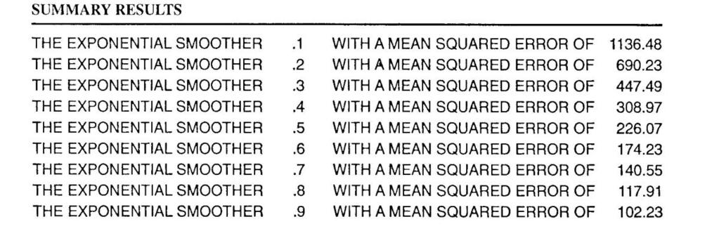
237 230

238 7.3 Regression Analysis for Sales and Earnings Projections What is regression analysis? Regression analysis is a statistical procedure for estimating mathematically the average relationship between the dependent variable and the independent variable(s). For example, regression analysis is used to estimate a dependent variable (such as cash collections from customers) given a known independent variable (such as credit sales). Simple regression involves one independent variable, price or advertising in a demand function, whereas multiple regression involves two or more variables, that is price and advertising together. First, we will discuss simple (linear) regression, defined by the following equation: Y = a + bx Where Y = dependent variable X = independent (explanatory) variable a = a constant or Y intercept of regression line b = the slope of the regression line How do I use the method of least squares? The method of least squares attempts to fine a line of best fit for the graph of a regression equation. To better explain this, let us define error, or u, as the difference between the observed and estimated values of sales or earnings. Symbolically, u = Y - Y' where Y = observed value of the dependent variable Y' = estimated value based on Y' = a + bx The least-squares criterion requires that the line of best fit be such that the sum of the squares of the errors (or the vertical distance in Figure 7.2 from the observed data points to the line) is a minimum, i.e., Mínimum: u 2 = (Y-a-bX) 2 231

239 Figure 7.2 Actual (Y) versus estimated (Y') Note: The objective of a scatter diagram is to demonstrate correlations. Each observation is represented by a dot on a graph corresponding to a particular value of X (the independent variable) and Y (the dependent variable). Also, you might want to make sure that a linear (straight-line) relationship existed between Y and X in the past sample. Using differential calculus we obtain the following equations, called normal equations: Solving the equations for b and a yields Y = na + b X XY = a X + b X 2 n XY - ( X)( Y) b = 2 2 n X ( X) a = Y bx where Y = ny and X = n X 232

240 Example 7.7 To illustrate the computations of b and a, we will refer to the data in Table 7.1. All the sums required are computed and shown below. Table 7.1 Original data and Computed Sums Advertising X (000) Sales Y (000) XY X 2 Y 2 $ $174 $225 3,414 2,792 4,359 From the table above: X = 174; Y = 225; XY = 3,414; X 2 = 2,792. X = X/n = 174/12 = 14.5; Y = Y/n = 225/12 = Substituting these values into the formula for b first: n XY - ( X)( Y) (12)(3,414) - (174)(225) b = = = n X ( X) (12)(2,792) - (174) 1,818 3,228 = a = Y - b X = (0.5632)(14.5) = = Thus, Y' = X 233

241 Assume that the advertising of $10 is to be expended for next year; the projected sales for the next year would be computed as follows: Y' = X = (10) = $ NOTE: Y 2 is not used here but rather is computed for r-squared (R 2 ). How can I use trend analysis? Trends are the general upward or downward movements of the average over time. These movements may require many years of data to determine or describe them. They can be described by a straight line or a curve. The basic forces underlying the trend include technological advances, productivity changes, inflation, and population change. Trend analysis is a special type of simple regression. NOTE: This method involves a regression whereby a trend line is fitted to a time series of data. The linear trend line equation can be shown as where t = time. Y = a + b t The formula for the coefficients a and b are essentially the same as the cases for simple regression. However, for regression purposes, a time period can be given a number so that t = 0. When there is an odd number of periods, the period in the middle is assigned a zero value. If there is an even number, then -1 and +1 are assigned the two periods in the middle, so that again t = 0. With t = 0, the formula for b and a reduces to the following: n ty b = 2 n t a= n Y EXAMPLE 7.8 Case 1 (odd number) 2X09 2X10 2X11 2X12 t =

242 Case 2 (even number) 2X07 2X08 2X09 2X10 2X11 2X12 t = In each case t = 0. Example 7.9 Consider ABC Company, whose historical sales follows. Year Sales (in millions) 2X08 $ 10 2X X X X12 17 Since the company has five years' data, which is an odd number, the year in the middle is assigned a zero value. Year t Sales(in millions (Y) ty t 2 2X08-2 $ X X X X b = (5)(18) 5(10) = 90/50 =1.8 a= 68 = Therefore, the estimated trend equation is Y' = $ $1.8 t To project 2X13 sales, we assign +3 to the t value for the year 2X13. Y' = $ $1.8 (3) 235

243 = $19 A summary of the four forecasting methods described in this chapter is provided in Figure 7.1. REMEMBER THIS: Use this table as a guide for determining which method is best for your specific circumstance. FIGURE 7.1 SUMMARY OF MORE COMMONLY USED FORECASTING METHODS 236

244 Chapter 7 Review Questions Section 1 1. Which one of the following is a sales forecasting technique? A. Linear programming (LP). B. Moving average. C. Queuing theory. D. Economic order quantity (EOQ). 2. The moving-average method of forecasting A. Is a cross-sectional forecasting method. B. Includes each new observation in the average as it becomes available and discards the oldest observation. C. Regresses the variable of interest on a related variable to develop a forecast. D. Derives final forecasts by adjusting the initial forecast based on the smoothing constant. 3. As part of a risk analysis, a manager wishes to forecast the percentage growth in next month s sales for a particular plant using the past 30 month s sales results. Significant changes in the organization affecting sales volumes were made within the last 9 months. The most effective analysis technique to use would be A. Unweighted moving average. B. Queuing theory. C. Exponential smoothing. D. Linear regression analysis. 4. A regression equation A. Estimates the dependent variables. B. Encompasses factors outside the relevant range. C. Is based on objective and constraint functions. D. Estimates the independent variable. 5. Regression estimation programs employ many tools for problem definition and analysis. A scatter diagram is one of these tools. The objective of a scatter diagram is to 237

245 A. Demonstrate correlations that make sure a linear (straight-line) relationship existed between Y and X in the past sample. B. Show frequency distribution in graphic form. C. Divide a universe of data into homogeneous groups. D. Show the vital trend and separate trivial items. 238

246 7.4 What Statistics to Look for in Regression Analysis A variety of statistics can be used to tell you about the accuracy and reliability of the regression results. We describe three in this section: 1. Correlation coefficient (R) and coefficient of determination(r 2 ) 2. Standard error of the estimate (S e ) and prediction confidence interval 3. Standard error of the regression coefficient (S b ) and t-statistic How can I measure the goodness of fit for the regression equation? The correlation coefficient R measures the degree of correlation between Y and X. The range of values it takes on is between -1 and +1. More widely used, however, is the coefficient of determination, designated R 2 (read as r-squared). Simply put, R 2 tells us how good the estimated regression equation is. In other words, it is a measure of "goodness of fit" in the regression. RULE of THUMB: The higher the R 2, the more confidence we have in our estimated equation. The coefficient of determination represents the proportion of the total variation in Y that is explained by the regression equation. It has the range of values between 0 and 1. EXAMPLE 7.10 The statement "Sales is a function of advertising expenditure with R 2 = 70 percent," can be interpreted as "70 percent of the total variation of sales is explained by the regression equation or the change in advertising and the remaining 30 percent is accounted for by something other than advertising, such as price and income." The coefficient of determination is computed as R 2 = 1 - (Y - Y' ) (Y - Y) 2 2 In simple regression situation, you can use this short-cut formula: R 2 = [n [n X 2 XY - ( X)( ( X) 2 ][n Y 2 Y)] - ( 2 Y) 2 ] Comparing this formula with the one for b, we see that the only additional information we need to compute R 2 is Y

247 Example 7.11 Refer to the table in Example 7.7. With Y 2, you can compute R 2 using the short-cut formula as follows: R 2 = 2 (1,818) = 2 [3,228][(12)(4,359) - (225) ] 3,305,124 = [3,228][52,308-50,625] 3,305,124 (3,228)(1,683) = 3,305,124 5,432,724 = = 60.84% INTERPRETATION: About percent of the total variation in sales is explained by advertising and the remaining percent is still unexplained. A relatively low R 2 indicates that there is a lot of room for improvement in our estimated forecasting formula (Y' = $ $0.5632X). Price or a combination of advertising and price might improve R 2. REMEMBER: A low R2 is an indication that the model is inadequate for explaining the y variable. The general causes for this problem are: 1. Use of a wrong functional form. 2. Poor choice of an X variable as the predictor. 3. The omission of some important variable or variables from the model. How can I measure the accuracy of management predictions? You can use the standard error of the estimate, designated Se, and defined as the standard deviation of the regression. The standard error of the estimate represents the variance of actual observations from the regression line. It is computed as: S e = (Y - Y' n - 2 ) 2 = Y 2 - a n - 2 Y - b XY This statistic can be used to gain some idea of the accuracy of our predictions. Example 7.12 Going back to our example data, S e is calculated as : S e = Y 2 - a Y - b XY = n - 2 4,359- ( )( 225)- (0.5632)(3,414) 12-2 = = 240

248 = Suppose you wish to make a prediction regarding an individual Y value--such as a prediction about the sales when an advertising expense = $10. Usually, we would like to have some objective measure of the confidence we can place in our prediction, and one such measure is a confidence (or prediction) interval constructed for Y. A confidence interval for a predicted Y, given a value for X, can be constructed in the following manner. Y' ± t S e (X X ( - X) 2 1 p 1 2 n X) 2 n where Y' = the predicted value of Y given a value for X; X p = the value of independent variable used as the basis for prediction. Note: t is the critical value for the level of significance employed. For example, for a significant level of (which is equivalent to a 95% confidence level in a two-tailed test), the critical value of t for 10 degrees of freedom is (See Table 7.3). As can be seen, the confidence interval is the linear distance bounded by limits on either side of the prediction. If you want to have a 95 percent confidence interval of your prediction, the range for the prediction, given an advertising expense of $10 would be between $10, and $21,836.10, as determined as follows: Note that from Example 4.2, Y' = $ The confidence interval is therefore established as follows: $ ± (2.228)(2.3436) ( ) (174) 2, = $ ± (2.228)(2.3436) (1.0764) = $ ± which means the range for the prediction, given an advertising expense of $10 would be between $ and $ Note that $ = $ and $ =$ How can I test the appropriateness of the regression coefficient? The standard error of the regression coefficient, designated S b, and the t-statistic are closely related. S b is calculated as: 241

249 S b = S e (X - X) 2 or in short-cut form S b = X 2 S e - X X) S b gives an estimate of the range where the true coefficient will "actually" fall. t-statistics (or t-value) is a measure of the statistical significance of an independent variable X in explaining the dependent variable Y. It is determined by dividing the estimated regression coefficient b by its standard error S b. It is then compared with the table t-value (See Table 7.3). Thus, the t-statistic measures how many standard errors the coefficient is away from zero. RULE OF THUMB: Any t-value greater than +2 or less than -2 is acceptable. The higher the t-value, the greater the confidence we have in the coefficient as a predictor. Low t-values are indications of low reliability of the predictive power of that coefficient. Example 7.13 The S b for our example is: S b = X 2 S e - X X) = 2, (14.5)(174) = ,792-2,523 = Thus, t-statistic = b S b = = CONCLUSION: Since, t = 3.94 > 2, we conclude that the b coefficient is statistically significant. As was indicated previously, the table's critical value (cut-off value) for 10 degrees of freedom is (from Table 7.3 at the end of the chapter). TO REVIEW: (1) t-statistic is more relevant to multiple regressions which have more than one b's. (2) R 2 tells you how good the forest (overall fit) is while t-statistic tells you how good an individual tree (an independent variable) is. 242

250 IN SUMMARY, the table t value, based on a degree of freedom and a level of significance, is used: (1) To set the prediction range upper and lower limits for the predicted value of the dependent variable. (2) To set the confidence range for regression coefficients. (3) As a cutoff value for the t-test. Figure 7.3 shows an Excel regression output that contains the statistics we discussed so far. FIGURE 7.3 EXCEL REGRESSION OUTPUT SUMMARY OUTPUT Regression Statistics Multiple R R Square (R 2 ) Adjusted R Square Standard Error (S e ) Observations 12 ANOVA df SS MS Significance F Regression Residual Total Coefficients Standard Error (S b ) t Stat Lower 95% Upper 95% Upper 95.0% Intercept Advertising (1) R-squared (R 2 ) = = 60.84% (2) Standard error of the estimate (S e ) = (3) Standard error of the coefficient (S b ) = (4) t-value = 3.94 All of the above are the same as the ones manually obtained. 243

251 7.4.1 Statistics to Look For In Multiple Regressions Multiple regressions are used to find the overall association between the dependent variable and explanatory (independent) variables. You need to take note of the following statistics when doing multiple regressions: t-statistics R-bar squared ( R ) and F-statistic Multicollinearity 2 Autocorrelation (or serial correlation) What does the t-statistics show? Even though the t-statistic was discussed in the previous section, we take it up again because it is more valid in multiple regression. The t-statistic shows the significance of each explanatory variable in predicting the dependent variable. In a multiple regression situation, the t-statistic is defined as t-statistic = b S i b i where i = i th independent variable RULE OF THUMB: It is desirable to have as large (either positive or negative) a t-statistic as possible for each independent variable. Generally, a t-statistic greater than +2.0 or less than -2.0 is acceptable. Explanatory variables with low t-value can usually be eliminated from the regression without substantially decreasing R 2 or increasing the standard error of the regression. Table 7.2 provides t-value for a specified level of significance and degrees of freedom. How do I measure goodness of fit? For multiple regressions, goodness of fit is best represented by R-bar squared ( R ): 2 2 R = 1 - (1 - R 2 ) n n 1 k where n = the number of observations k = the number of coefficients to be estimated An alternative test of the overall significance of a regression equation is the F-test. The F-statistic is defined as 244

252 F = (Y 2 (Y' Y) / k 2 Y') /(n k 1) Explained variation/k Unexplained variation/(n - k -1) If the F-statistic is greater than the table value, it is concluded that the regression equation is statistically significant in overall terms. NOTE: Virtually all computer programs for regression analysis show F-statistic. 2 R and How can I be sure the independent variables are unrelated? When using more than one independent variable in a regression equation, there is sometimes a high correlation between the independent variables themselves. Multicollinearity occurs when these variables interfere with each other. It is a pitfall because the equations with multicollinearity may produce spurious forecasts. Multicollinearity can be recognized when The t-statistics of two seemingly important independent variables are low The estimated coefficients on explanatory variables have the opposite sign from that which would logically be expected There are two ways to get around the problem of multicollinearity: One of the highly correlated variables may be dropped from the regression The structure of the equation may be changed using one of the following methods: o o o Divide both the left and right-hand side variables by some series that will leave the basic economic logic but remove multicollinearity Estimate the equation on a first-difference basis Combine the collinear variables into a new variable, which is their weighted sum What is autocorrelation (serial correlation)? Autocorrelation is another major pitfall often encountered in regression analysis. It occurs where there is a correlation between successive errors. The Durbin-Watson statistic provides the standard test for autocorrelation. Table 7.2 at the end of the chapter provides the values of the Durbin-Watson statistic for specified sample sizes and explanatory variables. Table 7.2 gives the significance points for d L and d U for tests on the autocorrelation of residuals (when no explanatory variable is a lagged endogenous variable). The number of explanatory variables, K excludes the constant term. Generally speaking, 245

253 Durbin-Watson Statistic Between 1.5 and 2.5 Below 1.5 Above 2.5 Autocorrelation No autocorrelation Positive Autocorrelation Negative Autocorrelation Autocorrelation usually indicates that an important part of the variation of the dependent variable has not been explained. WHAT TO DO: The best solution to this problem is to search for other explanatory variables to include in the regression equation. An example showing applications of all the tests discussed in this section can be found in Section Measuring the Accuracy of Your Forecasts The performance of a forecast should be checked against its own record or against that of other forecasts. There are various statistical measures that can be used to measure performance of the model. Of course, the performance is measured in terms of forecasting error, where error is defined as the difference between a predicted value and the actual result. Error (e) = Actual A - Forecast (F) What measures are commonly used for summarizing errors? Two measures are commonly used for summarizing historical errors: the mean absolute deviation (MAD) and the mean squared error (MSE). The formulas used to calculate MAD and MSE are MAD = e / n MSE = e 2 / (n - 1) The following example illustrates the computation of MAD and MSE. Example 7.14 Sales data of a microwave oven manufacturer are given below. Period Actual A Forecast (F) e (A-F) e e

254 Using the figures, MAD = e /n = 22/8 = 2.75 MSE = e 2 / (n - 1)= 76/7 = One way these measures are used is to evaluate forecasting ability of alternative forecasting methods. For example, using either MAD or MSE, a forecaster could compare the results of exponential smoothing with alphas and elect the one that performed best in terms of the lowest MAD or MSE for a given set of data. Also, it can help select the best initial forecast value for exponential smoothing. Note: Forecasting control can be accomplished by comparing forecasting errors to predetermined values or limits. Errors that fall within the limits would be acceptable while errors outside of the limits would signal corrective action to be desired. How do I choose the best forecasting equation? Choosing among alternative forecasting equations basically involves two steps. The first step is to eliminate the obvious losers. The second is to select the winner among the remaining contenders. How to eliminate Losers 1. Does the equation make sense? Equations that do not make sense intuitively or from a theoretical standpoint must be eliminated. 2. Does the equation have explanatory variables with low t-statistics? These equations should be reestimated or dropped in favor of equations in which all independent variables are significant. This test will eliminate equations where multicollinearity is a problem. 3. How about a low 2 R? The best candidates. A low 2 R can be used to rank the remaining equations in order to select the 2 R could mean: A wrong functional form was fitted An important explanatory variable is missing Other combinations of explanatory variables might be more desirable How to Choose the Best Equation 1. Best Durbin-Watson statistic. Given equations that survive all previous tests, the equation with the Durbin-Watson statistic closest to 2.0 can be a basis for selection. 247

255 2. Best forecasting accuracy. Examining the forecasting performance of the equations is essential for selecting one equation from those that have not been eliminated. The equation whose prediction accuracy is best in terms of measures of forecasting errors, such as MAD, MSE, RMSE, or MPE (to be discussed in detail in a later chapter) generally provides the best basis for forecasting. It is important to note that neither Lotus nor Quattro Pro calculate many statistics such as R-bar 2 squared ( R ), F-statistic, and Durbin-Watson statistic. You have to go to regression packages such as Statistical Analysis System (SAS), MINITAB, and Statistical Packages for Social Scientists (SPSS), to name a few. These packages all have PC versions. 7.6 How to Use a Computer Statistical Package for Multiple Regressions Are computers helpful for regression analyses? Software packages can greatly assist decision makers and forecasters with a variety of statistical analyses. How does the computer handle multiple regression? Here is an example of how a computer handles multiple regression. REMEMBER THIS: Each software package is a little different. For this example, we use SPSS, one of the most popular programs. In Figure 7.5, you will find a computer listing containing the input data and output results using three independent variables. To help you, illustrative comments have been added where applicable. EXAMPLE 7.15 Stanton Consumer Products Corporation wishes to develop a forecasting model for its dryer sale by using multiple regression analysis. The marketing department has prepared the following sample data that appear in the following table using three independent variables: sales of washers, disposable income, and savings. Sales of Disposable Sales of Washers Income Savings Dryers Month (X 1 ) (X 2 ) (X 3 ) (Y) January $45,000 $16,000 $71,000 $29,000 February 42,000 14,000 70,000 24,000 March 44,000 15,000 72,000 27,000 April 45,000 13,000 71,000 25,

256 May 43,000 13,000 75,000 26,000 June 46,000 14,000 74,000 28,000 July 44,000 16,000 76,000 30,000 August 45,000 16,000 69,000 28,000 September 44,000 15,000 74,000 28,000 October 43,000 15,000 73,000 27,000 Figure 7.5 SPSS Regression Output Model 1 Variables Entered/Removed b Variables Variables Entered Removed Method SAVINGS, sales, INCOME a. Enter a. All requested variables entered. b. Dependent Variable: SALESDRY Model 1 Model Summary b Std. Error Adjusted R of the R R Square Square Estimate Durbin-Watson.992 a a. Predictors: (Constant), SAVINGS, sales, INCOME b. Dependent Variable: SALESDRY Model 1 (Constant) sales INCOME SAVINGS Unstandardized Coefficients a. Dependent Variable: SALESDRY Coefficients a Standardi zed Coefficien ts B Std. Error Beta t Sig

257 1. The forecasting equation. From the SPSS output we see that Y' = -45, X X X 3 Suppose that in November the company expects X 1 = sales of washers = $43,000 X 2 = disposable income = $15,000 X 3 = Savings = $75,000 Then the forecast sales for the month of November would be Y' = -45, (43,000) (15,000) (75,000) = -45, , , ,375 = $27, The coefficient of determination. Note that the SPSS output gives the value of R, R 2, and R 2 adjusted. In our example, R = and R 2 = In the case of multiple regression, R 2 is more appropriate, as was discussed previously. 2 R = 1 - (1 - R 2 ) n n 1 k 10 = 1 - ( ) 10 = = = (9/7) This tells us that 97.5 percent of total variation in sales of dryers is explained by the three explanatory variables. The remaining 2.2 percent was unexplained by the estimated equation. 3. The standard error of the estimate (S e ). This is a measure of dispersion of actual sales around the estimated equation. The output shows S e = Computed t. We read from the output t-statistic X X X All t values are greater than a rule-of-thumb table t value of 2.0. (Strictly speaking, with n - k - 1 = = 6 degrees of freedom and a level of significance of, say, 0.01, we see from Table 15.3 that the table t value is ) For a two-sided test, the level of significance to look up was.005. In any case, we conclude that all three explanatory variables we have selected were statistically significant. 250

258 4. F-test. From the output, we see that F = (Y 2 (Y' Y) / k 2 Y') /(n k 1) Explained variation/k Unexplained variation/(n - k -1) = / / 6 = 9.703/0.082 = (which is given in the printout.) At a significance level of 0.01, our F-value is far above the value of 9.78 (which is from Table 7.4), so we conclude that the regression as a whole is highly significant. 6. Conclusion. Based on statistical considerations, we see that: The estimated equation had a good fit All three variables are significant explanatory variables The regression as a whole is highly significant The model developed can be used as a forecasting equation with a great degree of confidence 251

259 Table

260 253

261 TABLE

262 TABLE

263 256

264 Chapter 7 Review Questions Section 2 6. Correlation is a term frequently used in conjunction with regression analysis and is measured by the value of the coefficient of correlation, r. The best explanation of the value r is that it A. Interprets variances in terms of the independent variable. B. Is a measure of the relative relationship between two variables. C. Ranges in size from negative infinity to positive infinity. D. Is positive only for downward-sloping regression lines. 7. In regression analysis, the coefficient of determination is a measure of A. The amount of variation in the dependent variable explained by the independent variables. B. The amount of variation in the dependent variable unexplained by the independent variables. C. The slope of the regression line. D. The predicted value of the dependent variable. 8. In a simple linear regression model, the standard error of the estimate of Y represents A. A range of values constructed from the regression equation results for a specified level of probability. B. A variability about the least squares line that is uniform for all values of the independent variable in the sample. C. A measure of variability of the actual observations from the regression line. D. The proportion of the variance explained by the independent variable. 9. Multicollinearity occurs when A. A proportion of the variance is explained by the independent variable. B. Independent variables are correlated with each other. C. Observations are not independent. D. A random sample fails to represent the population. 10. Autocorrelation or serial correlation A. Means that observations are not independent. 257

265 B. Defines the proportion of the variance explained by the independent variable. C. Means that independent variables are correlated with each other. D. Is the failure of random samples to represent the population. 11. Two measures are commonly used for summarizing historical errors: the mean absolute deviation (MAD) and the mean. True or False? 258

266 Chapter 8: Making Use of Quantitative Decision Making Learning Objectives: After completing this section, you should be able to: Recognize the tools for decision making under conflict. Recognize the applications of linear programming to make optimize complex decisions. Identify techniques for inventory planning and control. Quantitative methods (or models) are used in operations research or management science. They refer to sophisticated mathematical and statistical techniques for solving problems pertaining to managerial planning and decision making. Numerous such techniques are available, eight of which are discussed in this chapter. They are: Decision making under certainty and conflict Decision making under uncertain conditions Decision theory Linear programming and shadow prices Learning curve Inventory planning and control Queuing models 259

267 8. 1 Decision Making under Risk, Certainty, and Conflict Decision making under risk involves decisions made when the probability of occurrence of the different states of nature is known. Decision making involves managing three major elements: Decision strategy. A decision maker implements a decision strategy which utilizes known existing organizational resources. States of nature. Elements of the environment over which the manager has little or no control. States of nature include the weather, political environment, economy, technological developments, etc. They can dramatically affect the outcome of any decision strategy. Outcome. The result of the interaction of the implementation of a decision strategy with the states of nature. Because of the variable nature of the states of nature, outcomes can be extremely difficult to forecast. Thus, outcomes of a decision strategy, O, the dependent variable, is a function of the interaction of the two independent variables, D, decision strategies and, S, the states of nature. Figure 8.1 shows a decision matrix, which is an approach to decision making under risk. Decision matrix, also called, payoff table, is a matrix consisting of the decision alternatives, the states of nature, and the decision outcomes. The rows are strategic choice a manager can make while the columns represent decision outcomes. An outcome O ij is a function of a decision strategy D i and state of nature S j. FIGURE 8.1 DECISION MATRIX States of Nature Strategies S 1 S 2 S 3.. S n D 1 O 11 O 12 * * * O 1n D 2 O 21 O 22 * * * O 2n D 3 * * *. * * *. D m O i1 O i2 * * * O mn Mathematically this relationship can be expressed as: Oi j f Di Sj where i=1,2, m and j=1,2, n. 260

268 What is decision making under certainty? This is the simplest type of decision making since it has a known state of nature. Therefore, the outcomes are the direct result of the chosen decision strategy, and can be predicted with certainty. In reality, this situation rarely occurs. The manager simply evaluates all the available decision strategies and then chooses the one best meeting the outcome criteria. Various optimization techniques can be utilized to maximize a decision strategy. Decision making under certainty occurs with problems that can be analyzed using basic inventory models, break-even analysis, linear programming, incremental analysis, and other methods where an outcome having one state of nature can be determined. What is decision making under conflict? In this situation, the decision maker is opposed by another party who is designing states of nature strategies to offset the decision maker s strategy to gain a competitive advantage. The decision maker must develop decision strategies to defeat an opponent s state of nature control strategy. This is the ideal setting for developing game strategies. Games are dependent on rules governing a competitive situation where the number of players, strategies, states of nature between the players, and degree of conflict control the outcomes. What are the types of games? Games are classified according to the degree of conflict of interest between the opponents. A zero sum game has a perfect inverse relationship between the gains and losses of the opponents. One opponent s gain is the other s loss. The total sum remains the same. In nonzero-sum games, the gains of one participant do not necessarily represent a comparable loss for the other party to the game. In the business environment, most competitive situations are nonzero-sum games. The prisoner s dilemma is a special outcome of a partly competitive game. In these games, each player has a strategy that dominates all others, and the outcome from each player s choice of his/her dominant strategy is less favorable to both players than some other outcome. How does a zero sum game work? 261

269 In a zero sum game the gains and losses are always equal. No player can gain more than the other player loses. Therefore, the game is always in equilibrium. The simplest type of zero sum game is the two-person zero sum game. Each player has a choice of game strategies. Since each player s gain will equal the other s loss, the outcome for each game strategy is known to each player. In the two-person zero sum game, the outcomes can be expressed numerically. A two-person zero sum game outcome matrix is show in Example 8.1. A positive number indicates a payoff to the player for rows A, and a negative number indicates a payoff to the player for columns B. In Example 8.1 the maximum any player can win/lose is 11. EXAMPLE 8.1 Two-player zero sum game outcome matrix Player B Player A Strategy F Strategy H r 1 r 2 Strategy D p 1 A wins 5 A wins 8 Strategy E p 2 A wins 6 B wins 2 (or A loses 2) What is a pure strategy? A pure strategy exists when there is one strategy for player A and one for player B that will be played every time. An equilibrium point is reached when it is at an optimum point for each respective player. This is termed a saddle point. A saddle point occurs where it is both the smallest numerical value in its row and the largest numerical value in its column. EXAMPLE 8.2 Example 8.2 shows a sample saddle point in a two-person zero sum game. Since 13 is the row minimum and the column maximum that is the saddle point strategy. The value of this game is 13. As the first choice Player A gains 13 while Player B loses 13. Saddle Point for two-person Zero Sum Game Player B Player A

270 8 4 7 What is a mixed strategy? When no player has one strategy that will be used each time, then there is no pure strategy used in the zero sum game. In this case the optimum point, or saddle point, is found using a mixed strategy. In this case, each player s strategy is chosen using a random number process. Nonetheless, one player s gain is another player s loss. EXAMPLE 8.3 Using the Two-Player Zero Sum Game Outcome Matrix in Example 8.1, it is possible to establish a mixed strategy. Assuming p 1 and p 2 are the probabilities for A s strategies, and n 1 and n 2 are the probabilities for B s strategies, their values can be determined using the following process in Section Decision Making Under Uncertain Conditions Under what conditions are decisions made? Decisions are made under certainty or under uncertainty (or risk). Under certainty implies that there is only one event and therefore only one outcome for each action. Under uncertainty, which is more common realistically, several events are involved for each action and with each a different probability of occurrence. WHAT TO DO: Under uncertainty, it is often helpful to compute the following: Expected value Standard deviation Coefficient of variation. What does expected value tell me? For decisions involving uncertainty, the concept of expected value ( r ) provides a rational means for selecting the best course of action. Expected value is defined as a weighted average using the probabilities as weights. It is found by multiplying the probability of each outcome by its payoff: r = r i p i 263

271 where r i is the outcome for i th possible event and p i is the probability of occurrence of that outcome. Note: A rational economic decision maker (one completely guided by objective criteria) will use expected monetary value to maximize gains under conditions of uncertainty because (s)he is riskneutral. Expected value represents the long-term average payoff for repeated trials. The best choice is the one having the highest expected value (sum of the products of the possible outcomes and their respective probabilities). What is the significance of the standard deviation? Whenever we talk about the expected value, one statistic that goes with it is standard deviation. Standard deviation is a statistic that measures the tendency of data to be spread out or is also a measure of the dispersion of a probability distribution. The smaller the deviation, the tighter the distribution, and thus, the lower the riskiness of the project. It is intuitively a margin of error associated with a given expected value. MBAs can make important inferences from past data with this measure. It is the square root of the mean of the squared deviations from the expected value ( r ). The standard deviation, denoted with the Greek letter To calculate, we proceed as follows:, read as sigma, is calculated as follows: 2 (r -r) p i i Step 1. First compute the expected rate of return (r ) Step 2. Subtract each possible return from r to obtain a set of deviations (r i - r ) Step 3. Square each deviation, multiply the squared deviation by the probability of occurrence for its respective return, and sum these products to obtain the variance ( 2 ): 2 = 2 (r -r) p i i Step 4. Finally, take the square root of the variance to obtain the standard deviation ( ). The standard deviation can be used to measure the variation of such items as the expected profits, expected contribution margin, or expected cash flows. It can also be used to assess the absolute risk associated with investment projects. RULE OF THE THUMB: The higher the standard deviation, the higher the risk. 264

272 What does the coefficient of variation mean? The coefficient of variation is a popular measure of relative dispersion, or relative risk. It represents the degree of risk per unit of return. It is computed by dividing the standard deviation by the expected value. EXAMPLE 8.4 /r Consider two investment proposals, A and B, with the following probability distribution of cash flows in each of the next five years: Cash Inflows Probability (.2) (.6) (.2) Project A $ Project B $ The expected value of the cash inflow is computed as follows: Project A Project B $200(.2) + 300(.6) + 400(.2) = $300 $100(.2) + 300(.6) + 500(.2) = $300 The standard deviations are computed as follows: For A: A = ($ ) 2 (.2) + ( ) 2 (.6) + ( ) 2 (.2) = $63.25 For B: B = ($ ) 2 (.2) + ( ) 2 (.6) + ( ) 2 (.2) = $ The coefficients of variation are computed as follows: For A: $63.25/$300=.21 For B: $126.49/$300=.42. CONCLUSIONS: Proposal B is more risky than proposal A since its standard deviation is greater. And, because the coefficient is a relative measure of risk, the degree of risk is also greater for Project B. 265

273 8.3 Decision Theory What is decision theory? Decision theory refers to a systematic approach to making decisions, particularly under conditions of uncertainty. While statistics such as expected value and standard deviation are essential for making your best choice, the decision problem can best be approached by using decision theory. Decision theory utilizes an organized approach such as a decision matrix (or payoff table). It is characterized by: The row: Each row represents a set of available alternative courses of action. The column. Each column represents the state of nature, or conditions that are likely to occur and over which you have no control. The entries. These appear in the body of the table and represent the outcome of the decision, known as payoffs. These may be in the form of costs, revenues, profits, contribution margins or cash flows. By computing expected value of each action, we will be able to pick the best one. EXAMPLE 8.5 Assume the following probability distribution of daily demand for strawberries: Daily demand Probability Also assume that unit cost =$3, selling price=$5 (i.e., profit on sold unit = $2), and salvage value on unsold units =$2 (i.e., loss on unsold unit =$1). The company can stock either 0, 1, 2, or 3 units. The problem is: How many units should be stocked each day? Assume that units from one day cannot be sold the next day. The payoff table can be constructed as follows: State of Nature Demand Expected value Stock (probability) (.2) (.3) (.3) (.2) 0 $ $0 Actions * **

274 *Profit for (stock 2, demand 1) equals (no. of units sold)(profit per unit) - (no. of units unsold)(loss per unit) = (1)($5-3) - (1)($3-2)= $2 - $1 = $1 **Expected value for (stock 2) is: -2(.2) + 1(.3) + 4 (.3) + 4 (.2) =$1.90 The optimal stock action is the one with the highest expected monetary value i.e., stock 2 units. What is the role of perfect information in decision theory? Suppose you can obtain a perfect prediction of which event (state of nature) will occur. The expected value with perfect information would be the total expected value of actions selected on the assumption of a perfect forecast. The expected value of perfect information (EVPI) can then be computed as: EVPI = Expected value with perfect information minus the expected value with existing information. EXAMPLE 8.6 From the payoff table in Example 8.5, with perfect information, you can make the following analysis: State of Nature Demand Expected value Stock (.2) (.3) (.3) (.2) 0 $0 $0 Actions $3.00 Alternatively, $0 (.2) + 2 (.3) + 4 (.3) + 6 (.2) = $3.00 CONCLUSIONS: The optimal stock action is stock 2, with the highest expected value of $1.90. Thus, with existing information, the best that you can do is to select stock 2 units to obtain $1.90. With perfect information (forecast), you could make as much as $3. Therefore, the expected value of perfect information (EVPI) = $ $1.90, or $1.10. This is the maximum price you should be willing to pay for additional information. Can you use a decision tree? 267

275 Decision tree is another approach used in discussions of decision making under uncertainty. It is a pictorial representation of a decision situation. As in the case of the decision matrix approach discussed, it shows decision alternatives, states of nature, probabilities attached to the state of nature, and conditional benefits and losses. The decision tree approach is most useful in a sequential decision situation. EXAMPLE 8.7 Assume XYZ Corporation wishes to introduce one of two products to the market this year. The probabilities and present values (PV) of projected cash inflows are given below: Product Initial investment PV of cash inflows Probabilities A $225, $450, , , B 80, , , , A decision tree analyzing the two products is given in Figure 8.2. FIGURE 8.2 Based on the expected NPV, choose product A over product B. NOTE: This analysis fails to recognize the risk factor in project analysis. 268

276 8.4 Linear Programming and Shadow Prices Linear Programming What is linear programming? Linear programming (LP) is a mathematical technique designed to determine an optimal decision (or an optimal plan) chosen from a large number of possible decisions. The optimal decision is the one that meets the specified objective of the company, subject to various restrictions or constraints. It concerns itself with the problem of allocating scarce resources among competing activities in an optimal manner. The optimal decision yields the highest profit, contribution margin (CM), or revenue, or the lowest cost. What does linear programming consist of? A linear programming model consists of two important ingredients: 1. Objective function. The company must define the specific objective to be achieved. 2. Constraints. Constraints are in the form of restrictions on availability of resources or meeting minimum requirements. As the name linear programming indicates, both the objective function and constraints must be in linear form. EXAMPLE 8.8 A firm wishes to find an optimal product mix. The optimal mix would be the one that maximizes its total profit or contribution margin (CM) within the allowed budget and production capacity. Or the firm may want to determine a least cost combination of input materials while meeting production requirements, employing production capacities, and using available employees. What are applications of linear programming? Applications of LP are numerous. They include: 1. Selecting least-cost mix of ingredients for manufactured products 2. Developing an optimal budget 3. Determining an optimal investment portfolio (or asset allocation) 269

277 4. Allocating an advertising budget to a variety of media. 5. Scheduling jobs to machines 6. Determining a least-cost shipping pattern 7. Scheduling flights 8. Gasoline blending 9. Optimal manpower allocation 10. Selecting the best warehouse location to minimize shipping costs. What is involved in the formulation of LP? To formulate an LP problem, certain steps are followed. They are: 1. Define what is called decision variables that you are trying to solve for. 2. Express the objective function and constraints in terms of these decision variables. NOTE: All the expressions must be in linear form. In the following example, we will use this technique to find the optimal product mix. EXAMPLE 8.9 The Omni Furniture Manufacturing Company produces two products: desk and table. Both products require time in two processing departments, Assembly Department and Finishing Department. Data on the two products are as follows: Products Available Processing Desk Table Hours Assembly hours Finishing Contribution Margin Per Unit $25 $40 The company wants to find the most profitable mix of these two products. Step 1: Define the decision variables as follows: A = Number of units of desk to be produced 270

278 B = Number of units of table to be produced Step 2: The objective function to maximize total contribution margin (CM) is expressed as: Total CM = 25A + 40B Then, formulate the constraints as inequalities: 2A + 4B < 100 (Assembly constraint) 3A + 2B < 90 (Finishing constraint) In addition, implicit in any LP formulation are the constraints that restrict A and B to be nonnegative, i.e., Our LP model is: A, B > 0 Maximize: Total CM = 25A + 40B Subject to: 2A + 4B < 100 3A + 2B < 90 A, B > 0 How do I solve LP problems? There are several methods available to solve LP problems. Here are two common ones: The simplex method. This is the most commonly used method of solving LP problems. It uses an algorithm, which is an iteration method of computation, to move from one solution to another until it reaches the best one. The graphical method. This solution is easier to use but limited to the LP problems involving two (or at most three) decision variables. To use the graphical method, follows these five steps: Step 1: Change inequalities to equalities. Step 2: Graph the equalities. To graph the equality, (1) set one variable equal to zero and find the value of the other and connect those two points on the graph and (2) mark these intersections on the axes and connect them with a straight line. Step 3: Identify the correct side for the original inequalities by shading. Repeat steps 1-3 for each constraint. 271

279 Step 4: After all this, identify the feasible region, the area of feasible solutions. Step 5: Solve the constraints (expressed as equalities) simultaneously for the various corner points of the feasible region. Determine the profit or contribution margin at all corners in the region. EXAMPLE 8.10 Using the data and the LP model from Example 8.9, obtain the feasible region (shaded area) by going through steps one through four. Then evaluate all of the corner points as follows: Corner Points Contribution Margin A B $25A + $40B (a) 30 0 $25(30) + $40(0) = $750 (b) (20) + 40(15) = 1,100 (c) (0) + 40(25)= 1,000 (d) (0) + 40(0) = 0 CONCLUSION: The corner, 20A, 15B produces the most profitable solution. (see Figure 8.3). FIGURE 8.3 THE FEASIBLE REGION AND CORNER POINTS 272

280 8.4.2 Shadow Prices (Opportunity Costs) What are shadow prices (opportunity costs)? If you have solved an LP problem, you might still wish to know whether it pays to add capacity in hours in a particular department. For example, you would be interested in the monetary value to the company by adding, say, an hour per week of assembly time. This monetary value is usually the additional contribution that could be earned. This amount is the shadow price of a given resource. Shadow prices constitute a form of opportunity cost if you consider it as the contribution margin that would be lost by not adding capacity. To justify a decision in favor of a short-term capacity decision, you must be sure that the shadow price exceeds the actual price of that expansion. For example, suppose that the shadow price of an hour of assembly capacity is $6.50 while the actual market price is $8.00. That means it does not pay to obtain an additional hour of the assembly capacity. Here is how to compute shadow prices (or opportunity cost): Add one hour (preferably, more than one hour to make it easier to show graphically) to the constraint of a given LP problem under consideration. 2. Resolve the problem and find the maximum CM. 3. Compute the difference between the CM of the original LP problem and the CM determined in step 2, which is the shadow price. EXAMPLE 8.11 Using the data in Example 8.10, we compute the shadow price of the assembly capacity. To make it easier to show graphically, add 8 hours of capacity of the assembly department, rather than one hour. The new assembly constraint and the resulting feasible region is shown in Figure 8.4. Then we evaluate all of the corner points in the new feasible region in terms of their CM, as follows: Corner Points Contribution Margin A B $25A + $40B (a) 30 0 $25(30) + $40(0) = $750 (b) $25(18) + 40(18)= 1,170 (c) 0 27 $25(0) + 40(227)= 1,080 (d) 0 0 $25(0) + 40(0) = 0 273

281 The new optimal solution, Corner b (18A, 18B) has total CM of $1,170 per week. The shadow price of the assembly capacity is $70 ($1,170 - $1,100 = $70), or $8.75 per hour ($70/8 hours = $8.75). YOUR CONCLUSION: The company would be willing to pay up to $70 to obtain an additional 8 hours of the assembly capacity per week, or $8.75 per hour per week. In other words, the company s opportunity cost of not adding an additional hour is $8.75. Figure 8.4 The Feasible Region And Corner Points How to Use the Computer for Linear Programming We can use a computer LP software package such as LINDO (Linear Interactive and Discrete Optimization) ( What's Best! ( or Microsoft Excel to quickly solve an LP problem. Figure 8.5 shows a computer output by an LP software program for out LP model. Figure 8.6 presents Excel LP solution. NOTE: The printout shows the following optimal solution: A = 20 units B = 15 units CM = $1,100 Shadow prices are: Assembly capacity = $8.75 Finishing capacity = $

282 Figure 8.5 The LP computer output Figure 8.6 The excel LP input and output 275

283 276

284 Chapter 8 Review Questions Section 1 1. A decision maker is operating in an environment in which all the facts surrounding a decision are known exactly, and each alternative is associated with only one possible outcome. The environment is known as A. Certainty. B. Risk. C. Uncertainty. D. Conflict. 2. One of your firm s trucks was involved in an accident with a car, and both parties claimed the other was at fault. A court ruled that your firm was solely responsible for all damage. From a game theory perspective, this dispute can be described as A. Prisoner s dilemma. B. Zero-sum game. C. Saddle point. D. Nonzero-sum game. 3. The expected value of perfect information is the A. Same as the expected profit under certainty. B. Sum of the conditional profit (loss) for the best event of each act times the profitability of each event occurring. C. Difference between the expected profit under certainty and the expected opportunity loss. D. Expected value with perfect information minus the expected value with existing information. 4. Management of a company has asked the internal auditing department to assist in determining whether a new automated system should be implemented and whether the supporting software should be developed in-house, purchased, or leased. This will require evaluating a sequence of alternatives, each of which will result in different outcomes. The most effective tool the company can use to evaluate these choices would be A. Ratio analysis. B. Decision matrix (payoff tables). C. Queuing theory. D. Decision tree. 277

285 5. A firm must decide whether to introduce a new product A or B. There is no time to obtain experimental information; a decision has to be made now. Expected sales can be classified as weak, moderate, or strong. How many different payoffs are possible in a decision tree under these circumstances? A. 2. B. 6. C. 3. D A firm wishes to find an optimal product mix. The optimal mix would be the one that maximizes its total profit or contribution margin (CM) within the allowed budget and production capacity. Or the firm may want to determine a least cost combination of input materials while meeting production requirements, employing production capacities, and using available employees. An appropriate technique for finding an optimal product mix is A. Linear programming. B. Capital budgeting. C. Differential analysis. D. Queuing theory. 7. Linear programming is an operating research technique that allocates resources. Mathematical expressions are used to describe the problem. The measure of effectiveness that is to be maximized or minimized is the A. Constraints. B. Set of decision variables. C. Objective function. D. Derivative of the function. 8. The constraints in a linear programming model are A. Included in the objective function. B. Costs. C. Scarce resources. D. Dependent variables. 278

286 9. Given the basic equations for the maximization of profits in a linear programming model, what quantitative technique is ordinarily employed to arrive at an optimal solution? A. Regression analysis. B. Markov analysis. C. Monte Carlo analysis. D. Simplex method analysis. 10. The graphic method as a means for solving linear programming problems A. Is limited to the LP problems involving two (or at most three) decision variables. B. Is limited to situations having two constraints. C. Is limited to situations with one constraint. D. Cannot be used with any constraints. 11. In linear programming, the shadow price refers to the A. Measurement of the value of relaxing a constraint in a problem with dual variables. B. Marginal change in profit associated with a change in the contribution margin of one of the variables. C. Unused capacity available once the optimal solution is obtained. D. Variables that are included in the final solution of the linear programming model. 279

287 8.5 Learning Curve How does the learning curve work to estimate labor hours? In manufacturing, labor hours are often observed to decrease in a definite pattern as labor operations are repeated. More specifically, as the cumulative production doubles, the cumulative average time required per unit will be reduced by some constant percentage, ranging typically from 10 percent to 20 percent. This reduction, and hence related costs, is referred to as the learning curve effect. How do I properly express the learning curve relationship? By convention, learning curves are referred to in terms of the complements of their improvement rates. For example, an 80 percent learning curve denotes a 20 percent decrease in unit time with each doubling of repetitions. EXAMPLE 8.12 Suppose that a project is known to have an 80 percent learning curve. It has just taken a laborer 10 hours to produce the first unit. Then each time the cumulative output doubles, the time per unit for that amount should be equal to the previous time multiplied by the learning percentage. An 80 percent learning curve is shown in Figure 8.7. Unit Unit time (hours) (10) = (8) = (6.4) = (5.12) = TAKE NOTE: As production quantities double, the average time needed per unit reduces 20 percent from its immediately previous time. 280

288 FIGURE 8.7 AN 80% LEARNING CURVE EXAMPLE 8.13 Big Mac Electronics Products, Inc. finds that new product production is affected by an 80 percent learning effect. The company has just produced 50 units of output at 100 hours per unit. Costs were as follows: Materials 50 $1,000 Labor and labor-related costs: Direct labor Variable overhead $2,000 The company has just received a contract calling for another 50 units of production. It wants to add a 50 percent markup to the cost of materials and labor and labor-related costs. To determine the price for this job, the first step is to build up the learning curve table. Quantity Total time (hours) Average time (per unit) hours (.8 x 2 hours) Thus, for the new 50 unit job, it takes 60 hours in total. The contract price is: Materials 50 $1,000 Labor and labor-related costs: Direct labor

289 Variable overhead $1, percent markup 800 Contract price $2,400 In what other ways can I use the learning curve? CHECKLIST OF APPLICATIONS FOR THE LEARNING CURVE The learning curve theory has found useful applications in many areas, including: 1. Budgeting, purchasing, and inventory planning 2. Scheduling labor requirements 3. Setting incentive wage rates 4. Pricing new products 5. Negotiated purchasing 6. Evaluating suppliers price quotations 8.6 Inventory Planning and Control Why are inventory planning and control important? One of the most common problems facing operations managers is inventory planning. This is understandable since inventory usually represents a sizable portion of a firm's total assets and, more specifically, on the average, more than 30% of total current assets in the U.S. industry. Excessive money tied up in inventory is a drag on profitability. The purpose of inventory planning is to develop policies which will achieve an optimal investment in inventory. You can do this by determining the optimal level of inventory necessary to minimize inventory related costs. Note: The ABC method of inventory control requires management to exert greatest control over the A classification items, which usually include a relatively small percentage of total items but a high percentage of the dollar volume. This method is analogous to the 80/20 rule, which says, for instance, that 20% of the customer s account for 80% of the profit. What kinds of costs are associated with inventory? Inventory costs fall into three categories. They are: 282

290 Ordering costs. These include all costs associated with preparing a purchase order, such as purchasing costs, shipping costs, setup costs, and quality discounts lost. Carrying (holding) costs. These include storage costs, handling costs, interest on capital invested, and obsolescence.. Shortage (stockout) costs. These are costs incurred when an item is out of stock. These include the lost contribution margin on sales plus lost customer goodwill. When and how much should I order? Several inventory planning models are available that try to answer these questions. Three such models are Economic order quantity (EOQ) Reorder point (ROP) Determination of safety stock. How does the Economic Order Quantity (EOQ) model work? The economic order quantity (EOQ) determines the order size that minimizes the sum of carrying and ordering costs. ASSUMPTIONS: Demand is assumed to be known with certainty and to remain constant throughout the year. Order cost is also known to be fixed. Also, unit carrying costs are assumed be constant. Since demand and lead time (time interval between placing an order and receiving delivery) are assumed to be determinable, no shortage costs exist. No quantity discounts are allowed. The EOQ is computed as: EOQ = 2DO C where C = carrying cost per unit, O = ordering cost per order, D = annual demand (requirements) in units. If the carrying cost is expressed as a percentage of average inventory value (say, 12 percent per year to hold inventory), then the denominator value in the EOQ formula would be 12 percent times the price of an item. NOTE: When an item is made instead of purchasing it, the EOQ model is used to determine the economic production run size where O = cost per setup. 283

291 EXAMPLE 8.14 Assume the Los Alamitos Store buys sets of steel at $40 per set from an outside vendor. It will sell 6,400 sets evenly throughout the year. The store's carrying cost is $8.00 per unit per year. The ordering cost is $100 per order. Therefore, 2(6,400)($100) EOQ = 160,000 = 400 sets $8.00 Total number of orders per year = D/EOQ =6,400/400 = 16 orders Total inventory costs = Carrying cost + Ordering cost = C x (EOQ/2) + O (D/EOQ) = ($8.00)(400/2) + ($100)(6,400/400) = $1,600 + $1,600 = $3,200 Based on these calculations, the Los Alamitos Store's inventory policy should be the following: (1) The store should order 400 sets of steel each time it places an order and order 16 times during a year. (2) This policy will be most economical and cost the store $3,200 per year. How do I determine the reorder point? Reorder point (ROP) tells you when to place a new order. However, this requires that you know the lead time from placing to receiving an order. Reorder point (ROP) is calculated as follows: Reorder point = (average demand per unit of lead time x lead time) + safety stock This tells you the level of inventory at which a new order should be placed. First, multiply average daily (or weekly) demand by the lead time in days (or weeks) yielding the lead time demand. Then add safety stock to this to provide for the variation in lead time demand to determine the reorder point. NOTE: If average demand and lead time are both certain, no safety stock is necessary and should be dropped from the formula. EXAMPLE 8.15 Using the previous example, assume lead time is constant at one week. There are 50 working weeks in the year. Then the reorder point is 128 sets = (6,400 sets/50 weeks) x 1 week. 284

292 CONCLUSION: When the inventory level drops to 128 sets, a new order should be placed. Suppose, however, that the store is faced with variable demand for its steel and requires a safety stock of 150 additional sets to carry. Then the reorder point will be 128 sets plus 150 sets, or 278 sets. Figure 8.8 shows this inventory system when the order quantity is 400 sets and the reorder point is 128 sets. FIGURE 8.8 BASIC INVENTORY SYSTEM WITH EOQ AND REORDER POINT When are these models realistic to use? The EOQ model described here is appropriate for a pure inventory system; that is, for single-item, singlestage inventory decisions for which joint costs and constraints can be ignored. EOQ and ROP assume that lead time and demand rates are constant and known with certainty. CAUTION: This may be unrealistic. Still, these models have been proved useful in inventory planning for many companies. There are, for instance, many businesses for which these assumptions hold to some extent. They include: Subcontractors who must supply parts on a regular basis to a primary contractor. Automobile dealerships, in which demand varies from week to week, but tends to even out over a season. CAVEAT: When demand is not known precisely and/or other complications arise, you should not use these models. You should instead refer to probabilistic models. What about Quantity Discounts? 285

293 EOQ does not take quantity discounts into account, which is often unrealistic in actual practice. Usually, the more you order, the lower the unit price you pay. A typical price discount schedule follows: Order quantity (Q) Unit price (P) 1 to 499 $ to or more WHAT TO DO: If quantity discounts are offered, you must weigh the potential benefits of reduced purchase price and fewer orders that will result from buying in large quantities against the increase in carrying costs caused by higher average inventories. Hence, the buyer's goal in this case is to select the order quantity which will minimize total costs, where total cost is the sum of carrying cost, ordering cost, and product cost: where P = unit price, and Q = order quantity. Total cost = Carrying cost + Ordering cost + Product cost = C x (Q/2) + O x (D/Q) + PD Use these steps to find economic order size with price discounts: EXAMPLE 8.16 Compute the common EOQ when price discounts are ignored and the corresponding costs using the new cost after discount. Compute the costs for those quantities greater than EOQ at which price reductions occur. Select the value of Q which will result in the lowest total cost. Using the information from the previous examples and the discount schedule shown previously, try to determine the EOQ. Recall that EOQ = 400 sets without discount. The total cost for this is: Total cost = $8.00(400/2) + $100(6,400/400) + $40.00(6,400) = $1,600 +1, ,000 = $259,200 The further we move from the point 400, the greater will be the sum of the carrying and ordering costs. Thus, 400 is obviously the only candidate for the minimum total cost value within the first price range. Q=500 is the only candidate within the $39.90 price range and Q=1,000 is the only candidate within the $39.80 price bracket. These three quantities are evaluated below and pictured in Figure

294 ANNUAL COSTS WITH VARYING ORDER QUANTITIES Order Quantity (Q) ,000 Purchase price (P) $40 $39.90 $39.80 Carrying cost (C x Q/2) $8 x (order quantity/2) $1,600 $2,000 $4,000 Ordering cost (O x D/Q) $100 x (6,400/order quantity) 1,600 1, Product cost (PD) Unit price x 6, , , ,720 Total cost $259,200 $258,640 $259,360 Note that C = $8.00, O = $100, and D = 6,400 for all possible orders. FIGURE 8.9 COSTS WITH QUANTITY DISCOUNT PROBLEM CONCLUSION: The EOQ with price discounts is 500 sets. The manufacturer is justified in going to the first price break but the extra carrying cost of going to the second price break more than outweighs the savings in ordering and in the cost of the product itself. What can I do when lead time and demand are uncertain? When lead time and demand are not certain, you must carry extra units of inventory, called safety stock, as protection against possible stockouts. To determine the appropriate level of safety stock size, you must consider the service level or stockout costs. Service level can be defined as the probability that demand will not exceed supply during the lead time. Thus, a service level of 90 percent implies a probability of 90 percent that demand will not exceed supply during lead time. Figure 8.10 shows a service level of 90%. 287

295 Here are three cases for computing the safety stock. The first two do not recognize stockout costs; the third does. Case 1: Variable demand rate, constant lead time ROP where = Expected demand during lead time + safety stock = u LT + z LT ( u ) u = average demand LT=lead time u =standard deviation of demand rate z = standard normal variate as defined in Table Normal Distribution table. For a normal distribution, a given service level amounts to the shaded area under the curve to the left of ROP in Figure FIGURE 8.10 SERVICE LEVEL OF 90 PERCENT EXAMPLE 8.17 Norman's Pizza uses large cases of tomatoes at an average rate of 50 cans per day. The demand can be approximated by a normal distribution with a standard deviation of 5 cans per day. Lead time is 4 days. Thus, u = 50 cans per day. LT= 4 days u = 5 cans How much safety stock is necessary for a service level of 99%? And what is the ROP? For a service level of 99%, z = 2.33 (from Table 8.1). Thus, 288

296 Safety stock = (5) = 23.3 cans ROP = 50(4) = cans FIGURE 8.11 SERVICE LEVEL OF 99 PERCENT Case 2: Constant demand, variable lead time ROP = Expected demand during lead time + safety stock where EXAMPLE 8.18 = u LT + z u ( LT ) u = constant demand LT = average lead time LT =standard deviation of lead time SVL's Hamburger Shop uses 10 gallons of cola per day. The lead time is normally distributed with a mean of 6 days and a standard deviation of 2 days. Thus, u = 10 gallons per day. LT = 6 days LT = 2 days How much safety stock is necessary for a service level of 99%? And what is the ROP? For a service level of 99%, z = Thus, Safety stock = 2.33 (10)(2) = 46.6 gallons ROP = 10(6) = gallons (note: z = 2.33 at 99% service kevel) Case 3: Incorporation of stockout costs This case specifically recognizes the cost of stockouts or shortages, which can be quite expensive. Lost sales and disgruntled customers are examples of external costs. Idle machine and disrupted production 289