A Macroeconomic Approach to a Firm's Capital Structure

Transcription

1 University of Pennsylvania ScholarlyCommons Publicly Accessible Penn Dissertations Summer A Macroeconomic Approach to a Firm's Capital Structure Mitsuru Katagiri mitsuruk@sas.upenn.edu Follow this and additional works at: Part of the Corporate Finance Commons, and the Macroeconomics Commons Recommended Citation Katagiri, Mitsuru, "A Macroeconomic Approach to a Firm's Capital Structure" (2011). Publicly Accessible Penn Dissertations This paper is posted at ScholarlyCommons. For more information, please contact libraryrepository@pobox.upenn.edu.

2 A Macroeconomic Approach to a Firm's Capital Structure Abstract In this paper, I investigate the logic behind cross sectional dispersion of firm's capital structure. I incorporate the trade off between tax benefits and financial distress costs into a dynamic general equilibrium model with heterogeneous firms and their endogenous entry/exit, and compute an equilibrium firm distribution. The main findings are summarized as follows. First, I find that the equilibrium distribution approximates the dispersion of firms' capital structure well. Second, I find that it simultaneously accounts for the relationship of capital structure to profitability \textit{and} firm size. The key mechanisms are the difference in responses to persistent and transitory productivity shocks and economies of scale. Third, I find through counterfactual experiments that even if the tax benefits do not exist, firms would not significantly change their capital structure in contrast to previous works. The intuition is that, with firm's entry/exit, young firms always exist and use debt until they accumulate internal funding. Degree Type Dissertation Degree Name Doctor of Philosophy (PhD) Graduate Group Economics First Advisor Jesus Fernandez-Villaverde Second Advisor Dirk Krueger Third Advisor Amir Yaron Keywords Corporate Capital Structure, Dynamic Tradeoff Theory, Heterogeneous Firm Model, Stationary Equilibrium, Firm Dynamics Subject Categories Corporate Finance Macroeconomics This dissertation is available at ScholarlyCommons:

3 A MACROECONOMIC APPROACH TO A FIRM S CAPITAL STRUCTURE Mitsuru Katagiri A DISSERTATION in ECONOMICS Presented to the Faculties of the University of Pennsylvania in Partial Fulfillment of the Requirements for the Degree of Doctor of Philosophy 2011 Jesus Fernandez-Villaverde Supervisor of Dissertation Dirk Krueger Graduate Group Chairperson Dissertation Committee Dirk Krueger, Ph.D. Professor of Economics Amir Yaron, Ph.D. Robert Morris Professor of Banking; Professor of Finance

4 c COPYRIGHT Mitsuru Katagiri 2011

5 To my parents iii

6 Acknowledgements First and foremost, I would like to express my deepest gratitude to my advisor, Professor Jesus Fernandez-Villaverde, for his constant support, guidance and encouragement. I am also grateful to my dissertation committee members, Professor Dirk Krueger and Professor Amir Yaron, for their valuable comments, encouragement, and discussion. Without their help, this dissertation could not be completed. I also thank to Professor Ufuk Akcigit, Professor Harold L. Cole, and Makoto Nakajima at Philly Fed for their helpful suggestions. I would also like to acknowledge graduate students at Penn. A special appreciation has to be expressed to Naoki Wakamori for continuous cheer and various supports. Also, I thank to my classmates, Naoki Aizawa, Nils Gornemann, Suryun Rhee, and Hikaru Saijo, for their suggestions in my practice for presentations, valuable comments to the project, and encouragements at every stage. Also, I would like to thank Hitoshi Mio, Shigenori Shiratsuka, and my colleagues at Institute for Monetary and Economic Studies at the Bank of Japan for their invaluable support. Without their deep understanding of my situation, I could not continue the project after I had returned to Japan. Finally, I would like to express my gratitude to my family for their support, encouragement, and shipment. I dedicate this work to my parents. iv

7 ABSTRACT A MACROECONOMIC APPROACH TO A FIRM S CAPITAL STRUCTURE Mitsuru Katagiri Jesus Fernandez-Villaverde In this paper, I investigate the logic behind cross sectional dispersion of firm s capital structure. I incorporate the trade off between tax benefits and financial distress costs into a dynamic general equilibrium model with heterogeneous firms and their endogenous entry/exit, and compute an equilibrium firm distribution. The main findings are summarized as follows. First, I find that the equilibrium distribution approximates the dispersion of firms capital structure well. Second, I find that it simultaneously accounts for the relationship of capital structure to profitability and firm size. The key mechanisms are the difference in responses to persistent and transitory productivity shocks and economies of scale. Third, I find through counterfactual experiments that even if the tax benefits do not exist, firms would not significantly change their capital structure in contrast to previous works. The intuition is that, with firm s entry/exit, young firms always exist and use debt until they accumulate internal funding. v

8 Contents Acknowledgements iv 1 Introduction 1 2 Related Literature Corporate Capital Structure Theories of Capital Structure Empirical Facts about Capital Structure Dynamic Trade Off Theory Macroeconomic Model with Firm Heterogeneity Firm s Life-Cycle, Entry/Exit, and Size Distribution Corporate Investment and Capital Structure Resource Misallocation and Macroeconomy Other Applicatioins Model Firms Technology Profit Evolution of the Firm s Balance Sheet Dynamic Optimization New Entrants Financial Intermediary Household Aggregation and Market Clearing Conditions Stationary Competitive Equilibrium vi

9 4 Stationary Equilibrium Calibration Results Distribution of Leverage Firm s Optimal Behavior Firm Size and Productivity Firm Age and Leverage Model Implication Relationship of Leverage to Firm Size and Profitability Joint Distributions of Firm s Characteristics Estimation Results The Logic behind the Estimation Results Cross Sectional Determinants of the Firm s Capital Structure What Makes Firms Use Debt? What Makes Firms Use Equity? Aggregate Effects of Tax Cut and Default Cost Corporate Income Tax Rate Default Cost Conclusion 92 A Algorithm to Compute a Stationary Equilibrium 94 B Algorithm for Numerical Experiment 95 C Data 96 vii

10 List of Tables 4.1 Calibration Tax Rates Estimate Results Changes in Average and Aggregate Leverage Changes in Average and Aggregate Leverage Changes in Aggregate Variables viii

11 List of Figures 3.1 Balance Sheet at the Beginning of Period Timing of Firm s Decision Histogram of Leverage (Data) Histogram of Leverage (Model) Policy Function of Asset Policy Function of Equity Policy Function of Leverage Policy Function of Lending Rate Distribution of Productivity and Asset Marginal Distribution of Asset Marginal Distribution of Productivity Marginal Distribution of Equity Firm Age and Leverage ROA and Employment Size (Data) ROA and Employment Size (Model) Leverage and Employment Size (Data) Leverage and Employment Size (Model) Leverage and ROA (Data) Leverage and ROA (Model) ix

12 Chapter 1 Introduction Many theoretical and empirical works have investigated the logic behind the distribution of corporate capital structures, which is widespread and stable over time, as one of central research topics in Corporate Finance for a long time. Modigliani and Miller (1958), a seminal classic paper in capital structure theory, argued that such a dispersion of leverage has nothing to do with firm s optimization. However, numerous empirical works have found that clear relationships between capital structure and other characteristics of firms such as size and profitability. 1 These empirical relationships suggest that firms ultimately choose their capital structure under some cost-benefit analysis. Given these stylized facts, theoretical works following Modigliani and Miller (1958) have investigated the cross sectional determinants of corporate capital structure. Among others, the dynamic trade off theory, which 1 For example, Frank and Goyal (2008) and Bernanke, Campbell, and Whited (1990) discuss the distribution of leverage in the U.S. data. Rajan and Zingales (1995) use G7 countries cross sectional data and investigate the cross sectional relationships of corporate capital structure to other corporate characteristics such as profitability and firm size. Fama and French (2002) and Frank and Goyal (2009) use the U.S. firm panel data and obtain similar results. Lemmon, Roberts, and Zender (2008) also uses the U.S. panel data and emphasizes the fixed effect of each firm. Graham and Harvey (2001) collects extensive survey data from CFOs of the U.S. firms and explore the key determinants of their capital structure decisions. 1

13 describes firms simultaneous choice of capital structure, investment, and payout under the trade off between tax benefits and financial distress costs, has succeeded in quantitatively accounting for the empirical facts. 2 While most papers based on the dynamic trade off theory are very recent and still not well-developed to explain some empirical facts, this theory is now the most promising one among theoretical models to quantitatively account for corporate capital structure. This paper constructs a structural model based on the dynamic trade off theory and investigate the following quantitative questions which have not been fully investigated by previous works. First, I examine whether the dynamic trade off theory can induce the widespread dispersion of corporate capital structure observed in data. I cannot answer this question by standard dynamic trade off models because most of them are partial equilibrium models focusing on a certain firm s optimal behavior, and deriving a cross sectional distribution in equilibrium is outside their scope. In order to overcome this shortcoming, I extend the model to a dynamic general equilibrium model with heterogeneous firms and their endogenous entry/exit. By doing so, I obtain not only an optimal policy for each firm, but also an equilibrium cross sectional distribution regarding firms characteristics. 3 Then I use the distribution as a natural counterpart of the empirical distribution for comparison. Second, I examine whether the trade off theory account for the relationship of corporate 2 A traditional static trade off theory was one of the most popular theories to describe corporate capital structure, but it was inconsistent with the negative relationship between firms leverage and their profitability observed in data. That is, according to the theory, profitable firms should increase their leverage because their probability of financial distress is low and their tax benefits are high. Recently, introducing a dynamic aspect into the trade off theory makes it possible to distinguish the internal equity from the outside equity and opens the door for the trade off theory to potentially explain the negative relationship. 3 Another way to obtain a cross sectional distribution in a structural model is to generate simulated data and construct a distribution by the data (e.g., Strebulaev (2007)). This approach does not consider the distribution itself as an equilibrium, but it is conceptually very similar to the stationary equilibrium approach in this paper. 2

14 capital structure to firm size and profitability. I focus on the relationship with those two variables because there is little disagreement on the relationships among empirical works. 4 In particular, I focus on the following stylized facts about the relationship: Fact 1 Correlation between profitability and firm size is positive Fact 2 Correlation between leverage and firm size is positive Fact 3 Correlation between leverage and profitability is positive, but it turns out to be negative if the data is limited to large firms Fact 4 Correlation between leverage and profitability becomes negative after controlling for firm size. As far as I know, the structural models to simultaneously account for these stylized facts do not exist. As potential mechanisms to explain those stylized facts, I incorporate the following two features into the dynamic trade off model, transitory and persistent idiosyncratic productivities and economies of scale. While these features are common in other literatures and justified by empirical works, they are not usually incorporated in dynamic trade off models. In a quantitative part of this paper, I test whether the combination of those two features and the trade off between tax benefits and financial distress costs quantitatively account for the stylized facts stated above. Finally, I measure a relative importance between cross sectional determinants of corporate capital structure. This question sounds a little bit ambitious because this is one of 4 In empirical works, a growth expectation measured by the market-to-book ratio is often considered as one of determinants, but there is no agreement on the sign of their effect on a book leverage among empirical works. For example, while Fama and French (2002) argues that it is positive, Rajan and Zingales (1995) and Lemmon, Roberts, and Zender (2008) argues that it is negative. Frank and Goyal (2009) shows the sign of the effect varies over time and concludes that it is not stable over time. 3

15 the most recurrent questions in the corporate finance literature. I give some answer to this question through counterfactual experiments. In the experiments, I drop frictions from the baseline model one by one and recalculate the equilibrium. Then I measure the effect of the friction on corporate capital structure by comparing the new equilibrium values with those in the baseline model. The main findings of this paper are summarized as follows. First, I find that the model s equilibrium distribution accounts for the dispersion of corporate capital structure observed in the data. In particular, it accounts for the two notable features in data. Many firms take very low leverage and the distribution is widespread. Second, I find that the equilibrium distribution also accounts for the stylized facts regarding the relationship of capital structure to firm size and profitability. In particular, it accounts for the four stylized facts stated above. The logic behind the result in the model is as follows. Fact 1 is induced just by the economies of scale. Fact 2 emerges in the model as a kind of spurious correlation. It is induced by the fact that firms with high persistent productivity get large and increase their leverage simultaneously. In the model, firms with high persistent productivity increase their leverage because, first, they invest more and expand their financing deficit and, second, the debt market is more accessible to them under the trade off. The first part of Fact 3 is induced by the combination of Fact1 and Fact2. To understand the logic behind the second part of Fact 3, the key mechanism is the difference between responses to the persistent and transitory productivity shock. Firms with a high persistent productivity increase their leverage as I explained above, but firms with a high transitory productivity decrease their leverage because their internal funding increases. Because the economies of scale caused by the fixed cost is not relevant for 4

16 large firms, only the latter negative effect remains when I measure the correlation between leverage and profitability using only large firm data. Similarly, Fact 4 is interpreted as follows: When I add firm size as another explanatory variable in addition to profitability, the firm size controls for the effect of the persistent productivity because firms with high persistent productivity get large. Thus, the profitability in the regression just captures the effect of transitory productivity, and have a negative effect on leverage. Finally, I discover the following implications about relative importance between determinants of capital structure through counterfactual experiments. First, even if the tax benefit does not exist, the aggregate and average leverage would not significantly change. This is in contrast to previous works. This contrast stems from the difference in the assumptions about firms entry/exit. That is, without firms entry/exit as a standard dynamic trade off model, all firms would eventually use 100% equity by accumulating their retained earnings when the tax benefit does not exist; but with firms entry/exit, young firms always exist and use debt in the process of accumulating their retained earnings. This result implies that the wedge in equity funding caused by the dividend tax and the flotation cost of equity are also important determinants of capital structure. This may answer the question why debt finance has been a pervasive funding way before the corporate income tax was introduced. 5 Second, the wedge in equity finance caused by the dividend tax and the flotation cost of equity has ambiguous effects on leverage. They actually depend on the firm s financial position and profitability. Rich and big firms decrease their leverage 5 Frank and Goyal (2008) says in their conclusion section that The U.S. corporate income tax did not begin until 1909 when it was introduced at a 1% rate. The use of debt contracts by businesses has a much longer history than does the corporate income tax. Thus, while taxes probably play an important role, there must be more to it. 5

17 while poor and small firms increase their leverage when the wedge in equity finance exists. Third, the default cost makes debt finance unattractive, but even if it is eliminated, the firm would continue to use some equity finance. Fourth, the investment irreversibility magnifies the disadvantage of debt finance, but it would have no effect on leverage if the wedge in equity finance did not exist. Fifth, corporate income tax cuts have large effects on aggregate variables such as output and capital accumulation. Sixth, the elimination of the default cost does not have significant effects on the aggregate variables. This implies that the effect of the default cost on aggregate variables may be overemphasized in previous literature. 6

18 Chapter 2 Related Literature In this chapter, I survey the literatures related to the main chapter of the Ph.D. thesis (called the current paper, hereafter). The objective of the current paper is to investigate cross sectional determinants of corporate capital structure using a heterogeneous firm model with the trade off between tax benefits and financial distress costs, and to conduct some policy experiments by the model. Roughly speaking, the current paper is related to two different literatures: One is corporate capital structure in corporate finance theory and the other is a macroeconomic model with firm heterogeneity. I review these two literatures one by one. 2.1 Corporate Capital Structure In this subsection, I review the papers about corporate capital structure choice. First, I select a small number of key classic papers in corporate capital structure theory. Some of them are not directly related to the current paper, but it is worthwhile to review them 7

19 because they are starting points of the investigation in corporate capital structure. Second, I review empirical papers about corporate capital structure. Since there are huge amount of empirical papers in this field, I choose the ones directly related to the current paper, and summarize the stylized facts established by them. Finally, I review papers belonging to the dynamic trade off literature. Since they are the most closely related works to the current paper, I review each of them in detail Theories of Capital Structure A starting point of the theoretical investigation in corporate capital structure is the irrelevance theorem by Modigliani and Miller (1958). It argues that as long as firms maximize just their value, the capital structure is irrelevant to their optimization problem. Because this theorem assumes that there are no frictions such as taxes, bankruptcy costs, agency costs, and asymmetric information, subsequent papers have tried to find out which frictions make corporate capital structure relevant to firms and investigate their implications. Frank and Goyal (2008) is a survey paper reviewing those theoretical developments. While many papers have been proposed, the trade off theory is one of the most accepted theories about corporate capital structure. It argues that firms choose their optimal capital structure given the trade off between the advantage and disadvantage of debt. The advantage of debt basically comes from taxes. Miller (1977) is a classic paper investigating the relationship between debt and taxes. He thinks of interest income taxation and dividend taxation as well as corporate income taxation, and derives formula about how tax benefits change along with the tax rates. On the other hand, the disadvantage of debt comes from financial distress costs such as default costs and fire sale costs. These 8

20 costs discourage firms to use debt, because when firms are in financial distress, they have to bear those costs to pay back interest and/or principal of debt. In the trade off theory, firms choose their capital structure under the advantage and disadvantage, and the current paper basically adopts the trade off as one of determinants of corporate capital structure. A testable implication of the trade off theory is that profitable firms are more leveraged because the tax benefits are big and the expected financial distress costs are low for profitable firms, but it is against the empirical evidence. I will review the empirical facts in the next subsection. The pecking order theory proposed by Myers (1984) is another accepted theory regarding corporate capital structure. It argues that firms prefer the internal funding the most, and when the internal funding is not enough to finance their investment, they issue debt. Only if firms cannot issue debt anymore because of the default risk or other financial distress costs, they issue equity. This theory is called the pecking order theory because of this strict hierarchy. He shows that this pecking order in capital structure choice is justified by asymmetric information between firms and investors as long as debt finance is less sensitive to information asymmetricity than equity finance. Stiglitz (1973) is the first paper investigating the effects of dividend taxation on corporate capital structure choice in a dynamic model. According to his model, with dividend taxation, firms financing behavior would be like the pecking order theory. The logic is simple. Firms prefer internal funding the most because using internal funding enables them to reduce dividends and cut back dividend tax payments. Also, firms would prefer debt to equity because issuing debt instead of equity means the profits will be distributed to bond holders rather than equity holders in the future, and then firms will be able to 9

21 cut back dividend tax payments. The current paper introduces the dividend taxation in the same manner, and the mechanism proposed in his model plays a key role to induce the pecking order behavior in the current paper too. Besides those major theories, there are many other models to explain corporate capital structure choice. Ross (1977) argues that the signalling effect of debt is a relevant determinant of capital structure. Since issuing debt sends a signal to investors that they are good firms, he argues that they choose their capital structure considering the signalling effect. Stulz (1990) focuses on the trade off caused by the conflict between equity-holders and managers. He argues that issuing debt prevents managers from diverting money to private benefits, but, on the other hand, it causes underinvestment. Brander and Lewis (1986) emphasize the interaction between corporate capital structure and production markets. They argue that in an imperfect competition environment, issuing debt works as a commitment to produce their products and carry benefits through the responses by other firms. Corresponding chapters of Tirole (2006) review those models in more detail Empirical Facts about Capital Structure Corporate capital structure is also one of central topics in empirical works. There are huge amount of empirical papers in this field, and so I choose and review the papers having direct implications to the current paper in this section. Then I extract the stylized facts established by them, and tell about the relations to the current paper. I start with the stylized facts about the distribution of leverage in raw data, which is one of main focus of the current paper. Frank and Goyal (2008) is a great survey summarizing the basic facts of the dispersion, and so I pick some facts which are closely related to the 10

22 current paper from the survey. As for the cross sectional dispersion of leverage, they show that many firms have very low leverage, say less than 10%. That is, many firms use no debt finance at all. On the other hand, while the number of firms tends to decrease as leverage increases, they also show that there exist firms taking more than 90% leverage. As a result, the distribution of leverage is very widespread. In the current paper, it is one of motivations whether the dispersion of leverage in the data can be replicated by an economic model. As for the time series movement of leverage, Frank and Goyal (2008) show that leverage in aggregate level is stationary over time, and remains around 30 %. This fact encourages us to use stationary equilibrium approach when we analyze corporate capital structure. Moreover, they compute the transition matrix of leverage and find that the time series movement of leverage in each firm level is also stable. That is, they show that firms with high (low) leverage tend to have high (low) leverage in the next period too. Lemmon, Roberts, and Zender (2008) also shows that high (low) levered firms tend to be high (low) levered for a long time. They use U.S. firm panel data in recent 40 years, and find that the autocorrelation process of corporate capital structure is very persistent over time, and most part of corporate capital structure can be explained by a time invariant fixed effect of each firm. While those papers do not compare the process of leverage with other processes, the autocorrelation of firm size measured by labor or asset is actually more persistent than that of leverage. Therefore, it is natural to guess that the leverage and firm size processes are governed by the same very persistent latent variable (i.e., firm s productivity) rather than there exist adjustment costs for rebalancing corporate capital structure. As I explained in the previous section, a number of theories are proposed to account for 11

23 the cross sectional determinants of corporate capital structure. Among others, the current paper is based on the trade off argument between tax benefits and financial distress costs, and so an important strand of empirical works is the estimation of these two things: the tax benefits and the financial distress costs. Graham (2000) is a seminal paper in the estimation of tax benefits. He estimates each firm s tax benefit, which is basically generated by the gap between tax rates on corporate income and personal interest income. He argues that because the estimated tax benefit is much bigger than conventional estimates of financial distress costs, it is difficult to justify corporate capital structure choices observed in data by the trade off. He also finds that large and profitable firms use debt conservatively, which is against the implication of trade off theory. A number of papers, on the other hand, estimate financial distress costs including default costs and fire sale costs. As for default costs, the world bank measures them all over the world and publishes the result as a part of Doing Business database. They basically accumulate fees for default procedures such as attorney fees and court fees, and conclude that the default cost in the U.S. is about 7% of the defaulted firm s estate. See Djankov, Hart, McLiesh, and Shleifer (2008) for how they construct the database. As for fire sale costs (i.e., the degree of investment irreversibility), there are some empirical works, but the estimation results vary across them a little. The lower bound is the estimate by Cooper and Haltiwanger (2006). They construct a structural model and estimate the discount rate of asset sale by indirect inference using plant level data in the U.S. The result is that firms discount the price of their assets like the machine for production by about 20% when they sell them. The upper bound is the estimate by Ramey and Shapiro (2001). They also estimate the discount rate of asset sale using aero space industry data. According to their estimation, the cost varies among the types of 12

24 assets, but it is around 60%. In the current paper, I use the default cost by the world bank and the median value of fire sale cost, say 40%. Finally, let me mention whether those financial distress costs are smaller than tax benefits for most firms as is argued by Graham (2000). In order to answer the question, it is important to estimate the marginal increase of default probability with respect to leverage ratio because we need to use expected financial distress cost for the comparison. However, it is not straightforward to estimate it because high leverage induces high default probability, but, at the same time, firms with low default probability tend to have high leverage. Molina (2005) estimates the marginal effect of leverage on the expected financial distress costs using some instrument variables, and shows that the marginal increases in expected financial distress costs is big enough to offset tax benefits. To investigate the cross sectional determinants of corporate capital structure, the most straightforward way is to ask firms about their financial strategy directly. Graham and Harvey (2001) collects survey data from CFOs of U.S. firms and investigate which determinants are relatively important for corporate capital structure choice. This survey contains a lot of results, so I pick several results relevant to the current papers. First, they find that financial flexibility and a good credit rating are the top two determinants of debt policy. They interpret financial flexibility as a precautionary motive related to future interest payment obligation and a good credit rating as an indication of their concern about financial distress costs. They also find that the financial flexibility is nothing to do with asymmetric information. Second, they find that firms do not care transaction costs when they issue debt. They argues that it is against the hypothesis by Fischer, Heinkel, and Zechner (1989). Third, they find that the following determinants do not seem 13

25 important: Conflict between bond-holders and equity-holders, conflict between managers and equity-holders, productioin market, and a debt level of competitors. Fourth, only a start-up firm considers equity as a cheap source of funds. All the results are just anecdotal evidences, but it is worthwhile to check whether the results of the current model do not contradict to those evidences. Next, I talk about the empirical relationships between capital structure and other firms characteristics such as firm size and profitability. These empirical relationships are just relationships between endogenous variables and do not directly tell anything about the cross sectional determinants, but they can be used in order to check the model validity by seeing whether the model can account for those empirical relationships or not. To investigate the empirical relationships, empirical researchers use firm level data in various countries and periods. For example, Rajan and Zingales (1995) uses G7 countries cross sectional data, and Fama and French (2002) and Frank and Goyal (2009) use the U.S. firm panel data of COMPUSTAT. They put slightly different set of variables in the regressions, but they regress the reduced form equation like the following one: Book Leverage i = β 0 + β 1 ROA i + β 2 log(employee i ) + β 3 Market-to-Book Ratio i + ϵ i ROA, the number of employees, and market-to-book ratio are used as proxies of profitability, firm size, and growth expectation, respectively. The empirical papers share the following estimation results: β 1 < 0 and β 2 > 0 That is, the coefficient on the profitability measured by ROA is negative and the coefficient 14

26 on the firm size measured by the number of employees (or asset size) is positive. The sign of the coefficient on the firms growth expectation measured by market-to-book ratio, β 3, is controversial. For example, while Fama and French (2002) argues that it is positive, Rajan and Zingales (1995) and Lemmon, Roberts, and Zender (2008) argues that it is negative. Frank and Goyal (2009) shows the sign of the relationship varies over time and concludes that the estimation result is not stable. Therefore, in the current paper, I just focus on the relationships of leverage to profitability and firm size, and use them as stylized facts to be explained. 1 The negative relationship between leverage and profitability has particularly received much attention from theoretical researchers because this negative relationship is puzzling in the light of the trade off theory. This is because the tax benefit is big and the probability of financial distress is low for profitable firms. Recently, introducing a dynamic aspect enables the trade off theory to potentially account for the negativity. I will talk about this dynamic trade off theory in the next section in detail. On the other hand, the other relationship, the relationship between leverage and firm size, is hardly analyzed by theoretical models, and, as a result, few models account for both relationships simultaneously. However, as Rajan and Zingales (1995) mentions, the magnitude of the negative relationship between leverage and profitability is much stronger for big firms than small firms. In the current papers, I also investigate such size dependency of the relationship between leverage and profitability. Finally, let me mention the empirical tests for the pecking order theory. The current paper does not incorporate the original version of the pecking order theory, which is induced 1 Tangibility of asset also has a clear positive relationship with leverage, but I do not mention tangibility of asset in the current paper because it is difficult to incorporate the concept of tangibility into the model. 15

27 by asymmetric information, but incorporate other mechanisms including dividend taxation to induce the pecking order behavior. Therefore, it is worthwhile to review those empirical papers about tests of the pecking order theory because they give some important and testable stylized facts. There are two key notions in the empirical investigation of the pecking order theory. The first one is financial deficit, which is defined as the investment minus the internal funding. 2 The pecking order theory argues that the financing deficit is filled by debt rather than equity. Shyam-Sunder and Myers (1999) tests this argument by the regressing the increase in debt on the financing deficit, and finds that the coefficient on the financing deficit is close to one, which is consistent with the pecking order theory. However, Frank and Goyal (2003) extends the data to small firms and conducts the Shyam- Sunder and Myers test. They find that the pecking order theory fits well for large firms, but poorly for small firms. That is, small firms use outside equity rather than debt to fill the financing deficit. Lemmon and Zender (2009) focus on debt capacity, which is the second key notion in this literature. The debt capacity is defined as the maximum amount of debt that the firm can borrow. Thus, when firms need to borrow more than the debt capacity, firms would use outside equity. They assume that firms with debt ratings have more debt capacity than firms with no debt ratings, because they are more accessible to public debt markets. They find that firms with no debt rating tend to issue outside equity by violating the pecking order when their financing deficit is large. Because firms with no debt ratings are usually small, rapid growth, young, and less profitable firms, their result is consistent with Frank and Goyal (2003). Leary and Roberts (2010) also get the same results regarding the characteristics of firms which violate the pecking order theory. They 2 Some people call it finaicial gap. 16

28 also find that the plain pecking order theory fits the data very poorly, but the fit drastically improves once controlling for other determinants proposed by the trade off theory. In sum, these empirical papers testing the pecking order theory give the following testable stylized facts: First, the financing deficit is basically filled by debt. Second, small, rapid growth, young, and less profitable firms tend to issue outside equity by violating the pecking order. It is worthwhile to check whether the implications of the current model do not contradict to these facts. Lastly, let me mention the implication of the fact that the financing deficit is mainly filled by debt. If this is the case, it would be difficult for the trade off model to account for the negative relationship between leverage and profitability. This is because profitable firms tend to invest more and expand their financing deficit, and then they have higher leverage. It means that it is much more demanding to account for the negative relationship between leverage and profitability under endogenous investment assumption than exogenous one. As I will state in the next section, most dynamic trade off models with adjustment costs of capital structure assume the exogenous corporate investment. Leary and Roberts (2005) estimates a hazard function of capital structure change, and argues that the costly rebalancing assumption can explain firms dynamic rebalancing of capital structure well after controlling for internal funding and investment expenditure. Therefore, it is not obvious whether the results established by the dynamic trade off models with exogenous investment are still valid under endogenous investment setting. 17

29 2.1.3 Dynamic Trade Off Theory In this section, I review papers belonging to the dynamic trade off literature, which is the most closely related literature to the current paper. Those papers have the following features in common. 1. Firms endogenously choose their capital structure under the trade off between tax benefits and financial distress costs, 2. Firms solve a dynamic optimization problem with uncertainty. The second feature makes this literature different from the traditional static trade-off models. As I explain below, introducing the dynamic aspect enables the trade off model to replicate some cross sectional stylized facts, which are considered as puzzling in the light of the traditional static trade off model. In particular, the negative relationship between leverage and profitability is considered as inconsistent with the trade off theory, but it is not necessarily inconsistent in a dynamic setting. In the rest of this section, I review the papers belonging to the dynamic trade off models one by one. Fischer, Heinkel, and Zechner (1989) is a pioneering paper in this literature. They assume that firms value exogenously follows a stochastic path, and given the firm value, firms choose their debt structure. Since they assume an adjustment cost for rebalancing the capital structure, firms capital structure does not respond until their leverage ratio reaches the upper or lower thresholds for recapitalization (so called, (s, S) inventory control problem). Thus, firms do not have a target value of leverage but have a target range of leverage, and, as a result, their leverage ratios change infrequently and swing over time as in data. 18

30 Strebulaev (2007) uses a similar model setting to Fischer, Heinkel, and Zechner (1989) and tries to replicate the negative relationship between leverage and profitability. He generates artificial panel data by similar quantitative method to the current paper and tests cross sectional implications including the relationship between leverage and profitability. A basic mechanism in his paper is that even though the firm s optimal leverage is positively correlated with its profitability, the actual leverage could be negatively correlated with its profitability because the leverage may deviate from its optimal level due to adjustment costs for rebalancing the capital structure. Unlike the current paper, the model cannot say anything about the relationship between firm sizes and leverage because corporate investment is totally exogenous. As a result, his paper cannot consider any effects of the financing deficit (gap between investment and internal fund) on leverage at all even though it is said to be an important determinant of capital structure in empirical papers. Therefore, it is not obvious whether the relationships replicated in his model are still valid under endogenous corporate investment. While most dynamic trade off models assume only a persistent stochastic shock to firms cash flow or value, Gorbenko and Strebulaev (2010) assumes a temporary shock in addition to a persistent shock as the current paper does. They focus on the fact that the volatility of asset value is much lower than that of cash flow, and shows that the temporary shock can induce the difference between these volatilities. The main contribution of their paper is that such volatile corporate earnings make debt riskier and less attractive than assumed in a standard dynamic trade off model, and resolve the low leveraged puzzle proposed by Graham (2000). The same effect is crucial to replicate low leverage in the current paper too, but, in addition to this effect, the temporary shock also plays a key role to replicate 19

31 the negative relationship between leverage and profitability in the current paper. Kurshev and Strebulaev (2006) focuses on the relationship between leverage and firm size as the current paper. They still assume exogenous investment and payout policy, but incorporate a fixed cost to adjust capital structure in addition to a proportional cost. As a result of the fixed cost, very small firms do not use debt at all in their model because the fixed cost to lever up is too expensive, and then those unleveraged small firms induce the positive relationship between leverage and firm size. On the other hand, the logic of the current paper to account for the positive relationship between leverage and firm size is much simpler: Productive firms optimally invest more and expand their size. At the same time, because those productive firms tend to have large financing deficit and are more accessible to debt markets, their leverage tend to be higher. All papers up to this point assume that corporate earnings, investment, and payout are totally exogenous. As I stated above, it is doubtful whether the results replicated by the models with the exogenous investment assumption are valid without the assumption because they do not consider the effect of financing deficit, which is said to be an important determinant of corporate capital structure. Hennessy and Whited (2005, 2007) are breakthrough papers in this literature because they assume endogenous investment and payout policy as well as endogenous capital structure choice. They assume a realistic tax system and financial distress costs, and account for the negative relationship between leverage and profitability under the trade off. The most important difference between their paper and the current paper is that their model is a partial equilibrium model focusing on a certain firm s optimal capital structure choice while the current paper is a general equilibrium model with entry/exit. Therefore, their model cannot consider the effect of firm evolution 20

32 on leverage, and it induces a significant difference in the results of counterfactual analysis. Also, since they do not consider the decomposition of productivity and economies of scale, it is likely that their model cannot replicate the relationship of leverage to profitability and firm size, simultaneously. Tserlukevich (2008) also replicates the negative relationship between leverage and profitability by the model with endogenous investment. In his model, firms investment responds to profitability shocks less frequently due to investment irreversibility, and so the positive profitability shocks just increase the equity value and decrease their leverage in many cases. Therefore, their leverage negatively correlated with their profitability even though firms lever up when they invest. His argument is theoretically clear, but obviously needs very severe investment irreversibility. The degree of investment irreversibility is 60% at most in empirical papers as I stated, but he assumes 100% investment irreversibility in the quantitative part of his paper. Thus, it seems difficult to quantitatively explain the negative relationship between leverage and profitability only by this mechanism. DeAngelo, DeAngelo, and Whited (2011) incorporates an exogenous debt capacity into a dynamic trade off model with endogenous investment and payout, and account for very conservative leverage behavior, which is consistent with Graham (2000). In their model, firms tend to keep their debt capacity for future funding needs because outside equity is more costly than debt. Thus firms do not completely fill their financing deficit by debt as in data. The current paper has the same mechanism, but the firm s debt capacity is endogenously determined in the current paper. That is, in the current paper, firms take a conservative leverage behavior because debt becomes more costly than internal and external equity funding as they lever up. 21

33 Finally, let me mention a criticism to the dynamic trade off models. Welch (2010) argues that dynamic trade off models should be tested by out-of-samples or quasi-experiments to validate their quantitative results in addition to in-sample moments. Moreover, he argues that it seems impossible for quantitative structural models like dynamic trade off models to specify all of the key determinants of corporate capital structure because there are so many determinants. He concludes that a simple reduced form model is more suitable for corporate finance than a complicated structural quantitative model. 2.2 Macroeconomic Model with Firm Heterogeneity Next I move on to the other literature related to the current paper: heterogeneous firm model. In the current paper, I adopt a general equilibrium model with heterogeneous firms as a baseline model, and then introduce a number of frictions including investment irreversibility, financial contract with costly defaults, and taxes. These frictions correspond to the ones assumed in a dynamic trade off theory, and make the capital structure relevant to firms optimization. There are two seminal classic papers in this literature. The first one is Hopenhayn (1992). He constructs a partial equilibrium model where each firm faces persistent idiosyncratic productivity shocks and chooses to stay or exit in every period. He proposes a concept of stationary equilibrium as an equilibrium concept of the economy. In the stationary equilibrium, each firm actively entries/exits and evolves in response to the idiosyncratic productivity shocks, but the whole economy is stationary over time and characterized by a time invariant distribution of firms (so called, a stationary distribution) because firms 22

34 entry/exit and expansion/shrink are offset each other. He shows that the stationary equilibrium with positive mass of firms entry/exist exists under some weak conditions. The other seminal paper in this literature is Hopenhayn and Rogerson (1993). They introduce a household sector into the Hopenhayn-model and extend the model to a dynamic general equilibrium model. A key assumption to characterize the stationary equilibrium in heterogeneous firm models is a decreasing return to scale of the production function. If the production function is constant return to scale as a standard neoclassical growth model, the most productive firm would keep all resources and any firm heterogeneity would not exit. In the current paper, I assume that the production function is decreasing return to scale according to this conventional wisdom. The rest of this section is organized as follows. First, I review the papers that account for some basic firms characteristics including their entry/exit, life-cycle, and size distribution by a heterogeneous firm model. Second, I focus on some papers that account for firms behavior towards corporate investment and capital structure like the current paper. Since they are very closely related to the current papers, I review each paper one by one in detail. Third, I review the papers about resource misallocation. The current paper is not directly related to the resource misallocation between firms, but I pick some seminal papers and review their motivation and contributions because it is the most growing literature for a heterogeneous firm model. Finally, I briefly review some other fields of study where a heterogeneous firm model is applied. 23

35 2.2.1 Firm s Life-Cycle, Entry/Exit, and Size Distribution Some stylized facts about firm heterogeneity in terms of the life cycle, entry/exit and size distribution have been established by micro data of firms. For example, Business Dynamics Statistics at the U.S. Census Bureau shows, for example, that the exit rates are higher for small and young firms than large and old ones, the firm size distribution is stable over time, young firms size distribution is more skewed rightward than that of old firms, and so on. Some empirical papers use other countries micro data of firms (e.g., Cabral and Mata (2003) for Portuguese data, Angelini and Generale (2008) for Italian data, and Mukoyama (2009) for Japanese data) to establish the stylized facts in those countries. Since Hopenhayn (1992) provides a great vehicle to think of firm heterogeneity, one of natural questions using his model is whether a heterogeneous firm model can account for those stylized facts. Some classic papers including Hopenhayn and Rogerson (1993) obtain results which are roughly consistent with those stylized facts, but some recent papers construct more sophisticated models and try to account for firms behavior more precisely. Atkeson and Kehoe (2005) investigates a firm s life cycle (that is, firms are born as small ones, grow as time goes on, and eventually exit from the economy) by an overlapping generation model with heterogeneous firms. In particular, they focus on the process of organization capital: the accumulated firm-specific knowledge. They show that their model can account for the age dependency of employment, job creation, and job destruction in the U.S. firms fairly well, and argue that the payment to the organization capital accounts for about 40% of payment to intangible assets. 24

36 Rossi-Hansberg and Wright (2007) investigates size dependency of firm s behavior by incorporating industry-specific human capital accumulation into a heterogeneous firm model. By doing so, the firm s technololy becomes decreasing return to scale with respect to capital, and, as a result, their model exhibits a mean reversion of firm s characteristics. Since this mean reversion induces the negative correlation between firm size and growth rate, their model obtains the result that the size distribution has thinner tails than Preto distribution particularly in capital intensive sectors as is observed in data. 3 Cooley and Quadrini (2001) investigates the size (age) dependency of firm s behavior among firms with the same age (size). First, they show that without any financial frictions or persistency of productivity shocks, firm s behavior would be independent of its age after controlling for its size. Next, they explicitly incorporate a debt contract with endogenous defaults between the financial intermediaries and firms. By doing so, firm s equity becomes a state variable in addition to its productivity because it has an effect on its credit availability. Then, as the firm age is correlated with the level of equity, the simultaneous dependencies emerge. 4 Methodologically, this is the first paper which incorporates financial intermediaries and one-period debt contract with endogenous defaults into a heterogeneous firm model. 5 Subsequent papers including Hennessy and Whited (2007), Gilchrist, Sim, 3 Even though the firm size distribution has thinner tails than Pareto distribution in data, there are a number of papers arguing that the firm size distribution theoretically has to follow Pareto distribution (so called, Zipf s law). See Luttmer (2010) for a survey of this literature. 4 There are some empirical papers about the relationship between firm size distribution and financial constraints. Cabral and Mata (2003) shows that the rightward skewness can be explained by financial frictions rather than a selection mechanism. Angelini and Generale (2008) show that financial frictions are significant determinants to account for the firm size distribution, particularly for small and young firms, but they also show that financial frictions have a limited explanatory power to a firm size distribution in financially developed countries like OECD countries. 5 It is common in business cycle literature to incorporate the same type of one-period debt contract into a dynamic general equilibrium model (e.g., Carlstrom and Fuerst (1997) and Bernanke, Gertler, and Gilchrist (1999)). Gale and Hellwig (1985) shows that the one-period debt contract would be optimal among general one-period contracts in a static model if there exists a monitoring cost (or a default cost), but, unfortunately, in a dynamic model with persistent shocks such as Cooley and Quadrini (2001) and 25

37 and Zakrajsek (2010) and the current paper utilize the contractual environment of a risky debt proposed by this model. Firm s entry and exit has been analyzed in a stationary setting, but its behavior over the business cycle attracts more attentions recently. Campbell (1998) is a classic paper about this topic. He describes that both entry and exit rates are positively correlated with business cycles, and, in particular, exit rates lead the productivity growth. He constructs a structural model and solves it by a linear-quadratic approximation, and then accounts for those pro-cyclicality. Samaniego (2008) constructs a similar heterogeneous firm model and solves it by nonlinear method. He considers a deviation from the stationary equilibrium as an aggregate productivity shock, and computes a deterministic transition path in which the economy returns to the stationary equilibrium. He documents that while entry and exit rates are pro-cyclical, the magnitude of their effects on aggregate variables including output and employment is negligible. It is very hard to incorporate an aggregate productivity shock into heterogeneous firm models with entry and exit because of the curse of dimensionality problem in general, but recently Clementi and Palazzo (2010) uses an approximation method proposed by Krussel and Smith (1998) to investigate the role of entry and exit over the business cycle, and finds out that firm s entry and exit amplifies the fluctuations in aggregate variables. While I assume that there is no aggregate shock in the current paper, it is a promising extension to incorporate the aggregate shock by using the method in their paper. the current paper, their result cannot be directly applied. Thus, as long as I know, it is an open question whether a debt contract is optimal in those models. 26

38 2.2.2 Corporate Investment and Capital Structure The most closely related application field of heterogeneous firm models to the current paper is the literature of corporate investment and capital structure. Gomes (2001) investigates whether financial constraints induce the cash flow effect in corporate investment. He constructs a heterogeneous firm model with entry and exit and incorporates a flotation cost of equity as a financial constraint. He derives a stationary distribution in the equilibrium, and then randomly generates artificial cross sectional data from the distribution for comparison with the empirical results. He concludes that the cash flow effect on investment is nothing to do with financial constraints, but caused just by measurement errors. The current paper actually uses the same quantitative methodology to test cross sectional implications. Khan and Thomas (2008) investigates why the aggregate investment over business cycles is relatively smooth while the investment of individual firm is lumpy. They show that the aggregate investment is as lumpy as the investment of individual firms in a partial equilibrium model, but this lumpiness in the aggregate investment disappears when the model is extended to a general equilibrium model because general equilibrium effects dampen the response of investment. Methodologically, this is the first paper which incorporates an aggregate productivity shock into heterogeneous firm models. They basically apply the method proposed by Krussel and Smith (1998). The method used in their paper to approximate the aggregate state is adopted in subsequent papers including Bloom, Floetotto, and Jaimovich (2010) and Gomes and Schmid (2010). Miao (2005) investigates corporate capital structure and entry/exit behavior by the stationary equilibrium approach as the current paper. He constructs a general equilibrium 27

39 model with endogenous corporate capital structure choice and default, and accounts for some stylized facts and conducts counterfactual experiments. This paper is the most closely related to the current paper in the sense of motivation, but, unlike the current paper, he makes several drastic simplifications to obtain closed form solutions. For example, he assumes a perpetual bond which pays a fixed amount of coupon, and the amount of the bond is fixed after they enter the economy. Moreover, he considers only a corporate income tax as a relevant tax for firms, and assumes that firms never choose to pay dividends. The current paper, on the other hand, focuses on quantitative solutions under more realistic circumstance while it does not give closed form solutions. 6 Gomes and Schmid (2010) investigate credit spreads, equity premium, and capital structure simultaneously by a heterogeneous firm model with aggregate productivity shocks. They extend a standard heterogeneous firm model with entry and exit so that firms endogenously choose their capital structure. At the same time, however, they abstract from many aspects for simplicity. For example, they assume that the size and structure of firms balance sheet is fixed once it is decided when firms enter the economy. They show that the model accounts for the level of credit spread as well as corporate leverage, equity premium, and business cycle statistics. Their result implies that aggregate productivity shocks play an important role to explain those things simultaneously. The current paper can define credit spreads inside the model too, but since the current paper does not incorporate an aggregate shock, it is not surprising that it cannot account for the level of credit spread. 6 In the conclusion part of his paper, he said that introducing a dynamic capital structure choice as the current paper does is one of promising future extensions of his paper. 28

40 2.2.3 Resource Misallocation and Macroeconomy As some empirical papers show, resource allocation is an important aspect to account for the measured TFP in a whole economy. In response to the accumulation of such empirical evidences, resource (mis)allocation is now becoming one of the most growing literatures for heterogeneous firm models. I discuss the literature in two parts below: resource misallocation by financial allocation and that by other reasons. As for the resource misallocation due to financial frictions, Buera and Shin (2010) explores how financial frictions affect the convergence to the steady state economy. They construct a heterogeneous agent model with an occupational choice: people can either produce by their own technology or work as a labor force. They consider the case that the resource is misallocated by some distortions such as taxes or other government policies in the initial state. They show that the economy would converge to a new steady state when the distortions are eliminated, but financial frictions slow down the speed of the convergence. This is because, with financial frictions, people need to accumulate the assets for collateral use in order to fund for production. Buera, Kaboski, and Shin (2011) investigates the difference in TFP between developed and developing countries. In particular, they focus on the fact that the difference in TFP is bigger in the sector where the economy of scale is large. They use an occupational choice model similar to Buera and Shin (2010), and extend it to two-sector model, where these sectors are different in terms of the degree of scale economy. Their main argument is that financial frictions are more relevant in the sector with large scale economy like the manufacturing sector because people need to use more capital for producing their products 29

41 efficiently. Therefore, since people with high ability cannot operate due to the financial friction, TFP would be depressed through talent misallocation. Moll (2010) constructs a heterogeneous agent model with collateral constraint and accounts for the output difference between countries with different degree of financial frictions. In particular, in his model, the persistence of idiosyncratic productivity shocks plays a key role to determine the effect of financial frictions. If it s not persistent, financial frictions do not have any effects on capital allocation and aggregate output because people can finance their investment by their own savings eventually. Midrigan and Xu (2010) also investigates the relationship between aggregate TFP and resource misallocation. In particular, they focus on how much the misallocation is quantitatively explained by financial frictions. They construct a heterogeneous agent model where people are forced to fund their operational costs in advance, and incorporate financial frictions as a collateral constraint. They show that the financial friction could generate the big difference in TFP, but under plausible calibration values, the TFP difference through the misallocation caused by the financial friction in their model is too small to account for the TFP difference in data. 7 As for the resource misallocation due to other reasons, Hopenhayn and Rogerson (1993) investigates how the introduction of a firing tax affects the aggregate variables such as output and labor productivity. They calibrate the model without the firing tax by U.S. micro data, and then introduce the firing tax and compare the stationary equilibriums before and after the introduction of the tax. They show that the firing tax decreases output through decrease in employment because the firing tax increases the labor cost. 7 This result is consistent with Buera and Shin (2010), which argues that it is impossible to generate the difference in TFP between developed and developing countries only by financial frictions. 30

42 Also, and more importantly, the firing tax decreases output through decline in productivity too because the firing tax disrupts smooth reallocation of labor force between firms. As a whole, while introduction of the firing tax reduces the fluctuation of employment, it induces a substantial decrease in output. Restuccia and Rogerson (2008) investigates how resource distortions induce decline in measured TFP by a very standard heterogeneous firm model with capital and labor. They introduce output taxation as a source of distortion and see its effect on TFP and output. First, they show that if the tax rate is uncorrelated with idiosyncratic productivity, the distortion is not that big, but if it is positively correlated (i.e., productive firms are taxed more), the distortion is pretty big. For example, when the tax rate is equal to 40%, the uncorrelated distortion induces just 8% decline in TFP, but the correlated distortion induces 31% decline in TFP. Gourio (2008) investigates the effect of reallocation induced by removal of a capital adjustment cost. In particular, he emphasizes how much the effect changes if firm s productivity process is incorrectly specified. He constructs a heterogeneous firm model with permanent, persistent and transitory idiosyncratic productivity shocks. He utilizes the fact that corporate investment responds to the persistent shocks rather than the transitory shocks to identify those productivity shocks by micro data, and estimates the model parameters by the simulated method of moment. He puts those estimated parameters into a general equilibrium model with firm heterogeneity, and show that the difference in specification of the productivity process significantly affects the effect of the removal of a capital adjustment cost. 31

43 2.2.4 Other Applicatioins There are some other fields of study where heterogeneous firm models are used. The first field is firm s pricing behavior. Golosov and Lucas (2007) investigates the price stickiness observed in data by incorporating an adjustment cost for changing prices (i.e., a menu cost). They argue that their model is more natural than Calvo-type model because, in their model, firms with prices far from the optimal level tend to change the prices while, in Calvo-type model, firms change the prices regardless of their current prices. They show that the effect of monetary policy on output in their model is much smaller than that in the model with Calvo-type price setting (e.g., New Keynesian model) because of this selection mechanism. Midrigan (2010) also measures the effect of monetary policy by a heterogeneous firm model with a menu cost. He shows that Golosov and Lucas (2007) cannot account for heterogeneity in the size of price changes and temporary price changes. In order to replicate those features, first, he assumes two types of prices: regular prices and posted prices. Then he also assumes a scale economy only for the regular price change and a fat-tail distribution for idiosyncratic cost shocks. These assumptions not only enable the model account for those features, but also induce a much bigger effect of monetary policy than that in a standard menu cost model. This is because, first, there are fewer firms around the threshold when the distribution of cost shocks has a fat-tail, and second, a scale economy makes the size of most price changes smaller. The second field is about the uncertainty shock. Bloom (2009) defines the uncertainty 32

44 shock as changes in volatility of idiosyncratic productivity shocks of each firm, and investigates their effect on aggregate labor and output. First, he shows by VAR that the uncertainty shock induces a sharp decline in a short term and an overshoot in a medium term in output and aggregate employment. Then he constructs a heterogeneous firm model with investment and labor irreversibility, and shows that the model accounts for the response to the uncertainty shock. The intuition of the sharp decline is that increases in volatility expand the inaction area caused by the irreversibility, and, as a result, decrease Solow residual due to misallocation between plants. On the other hand, because increases in volatility enhance the fraction of firms outside the inaction region, they increase mediumterm employment and generate output overshoot. The third field of application is a trade theory. Melitz (2003) investigates the effect of trade on the welfare and aggregate productivity. He extends a heterogeneous firm model with firm s entry/exit to a trade model with monopolistic competition, and compares the economies with and without a trade opportunity. The main result is that the aggregate productivity and welfare would improve through reallocation between firms when the trade is available for firms. The intuition is as follows: When the trade becomes available, only productive firms expand their share by exporting their products because exporting products is assumed to be costly. On the other hand, less productive firms produce just for the domestic market and shrink their share, or they exit if their expected profit is negative. As a result, with the trade opportunity, more productive firms produce more, and then the aggregate productivity and welfare would improve through the reallocation. The fourth, and last, field of application is public finance. Gourio and Miao (2010a,b) 33

45 simultaneously incorporate corporate income tax, capital gain tax, dividend tax, and income tax into a heterogeneous firm model, and quantify the effect of dividend tax reform introduced in the U.S. in Gourio and Miao (2010a) investigates the effect of the permanent change in the dividend and capital gain tax, and argues that the U.S. tax reform increased a long-run capital stock by about 4%. They show that firm heterogeneity is important for precisely measuring the effects of tax reforms because the dividend tax affects long-run capital accumulation through changes in capital allocation between firms. They also show that if they ignore the general effect, the effect on capital accumulation would become about six-times larger. Gourio and Miao (2010b) extends Gourio and Miao (2010a) by incorporating a risky debt in addition to equity and model the endogenous choice of corporate capital structure. 8 Then they investigate the effect of the temporary tax cut and its transitional dynamics. 8 While they assume tax deductibility of interest payments, they do not incorporate any financial distress costs into the model but just assume the collateral constraint. Therefore, unlike the current paper, there is not the trade-off between tax benefits and financial distress cost associated with the debt financing in their model. 34

46 Chapter 3 Model The model is based on a dynamic general equilibrium model with heterogeneous firms and their endogenous entry/exit like Hopenhayn and Rogerson (1993) and Gomes (2001). In the model, each firm is hit by idiosyncratic productivity shocks, but not aggregate productivity shocks. By this assumption, the model has a competitive equilibrium with a stationary distribution regarding firm s characteristics. In a quantitative part, I consider this stationary distribution as a counterpart of cross sectional data in the real economy, and explore the logic behind the stylized facts using artificial data generated from the stationary distribution. 1 The economy consists of three types of agents: firms, households and financial intermediaries (FI). The firm produces consumption goods by asset and labor in every period. It finances the asset by three financing sources. The first one is an internal funding generated by the accumulation of their profit. The second one is outside equity coming from 1 As Frank and Goyal (2008) states, the aggregate leverage ratios is very stable over time. This fact justifies the assumption that there is no aggregate shock. 35

47 the household through an equity market. The third one is a business loan from the FI. Note that the first two sources are listed as equity and the third one is listed as debt in a liability side of its balance sheet. As a result of its optimal choices between the three financing sources, the capital structure is determined endogenously in the model. The household is homogeneous and infinitely lived, and maximizes the lifetime utility by consumption and labor supply. The household s financial asset consists of the share of the firm and the risk-free deposit at the FI. The income consists of wages, dividends on the share and interests on the deposit. The household uses the income to buy consumption goods and new shares, and the rest is deposited at the FI at the risk-free rate. The last agent in the model is the FI. It collects deposit from the household at risk-free rate and lend it to the firm as a business loan. Since I assume a competitive FI market, the FI s expected profit is zero. 2 As to the financial contract between the FI and the firm, I limit the contract space to a standard one-period debt contract with default costs as in Cooley and Quadrini (2001) and Hennessy and Whited (2007). I do not show that a simple one-period debt contract is an optimal contract in this model setting, but the fact that it is one of the most common financial contracts in the real economy justifies the assumption. 3 2 Actually, since I focus just on a stationary economy, the ex-post FI s profit is also always equal to zero due to a law of large number. 3 Limiting the contract space to a one-period debt contract significantly simplifies the model, but excludes the following more general contract schemes from the contract space in the first place. First, I exclude a dynamic lending contract under asymmetric information as in Clementi and Hopenhayn (2006) and Quadrini (2004). Second, I exclude one-period financial contracts outside a debt-contract. Gale and Hellwig (1985) shows that a debt contract would be optimal among general one-period contracts if information frictions between lenders and borrowers and a monitoring cost (or a default cost) exist, but, unfortunately, I cannot directly utilize their result because the current model is a dynamic model with persistent idiosyncratic shocks while their model is a static model. 36

48 3.1 Firms There is a continuum of firms producing final goods by asset and labor. In every period, after the firm produces final goods, it has the following three choices: continue the business, exit from the economy or default on its loan. There is also a continuum of new entrants. When they enter the economy, their initial productivity is drawn from some distribution. Given the initial productivity, the new entrants decide whether they stay or immediately exit from the economy without producing anything. In a stationary equilibrium, the distribution of firm s characteristics is stationary in the sense that it does not change before and after the firm s entry/exit because their entry/exit is offset each other Technology The firm uses two inputs, asset, k, and labor, l, to produce consumption goods. As to its technology, I assume a standard Cobb-Douglas production function, y = zk α k l α l. I assume diminishing return to scale, α k + α l < 1. 4 z is an idiosyncratic productivity to each firm. This idiosyncratic productivity consists of two parts: persistent component, z p, and transitory component, η. z z p η 4 This assumption makes a firm size matter. If the technology is constant return to scale and there is heterogeneity in firm s productivity, it would be efficient that the firm with the highest productivity uses all asset and labor, and the firm s distribution would be degenerate. 37

49 The persistent part follows the AR(1) process after log-transformation, log(z p,t ) = ρ log(z p,t 1 ) + ϵ t where ϵ t N(µ ϵ, σ ϵ ) (3.1) and produces the heterogeneity in characteristics of firms such as size and capital structures. The transitory component, on the other hand, follows a Normal distribution after logtransformation. log(η t ) N(0, σ η ) Profit A competitive consumption goods market is assume. As a result, the price level of the consumption goods is the same for all firms, and it is normalized to one. Then the revenue (i.e., the price times the amount of sale) is equal to the amount of sale, zk α kl α l. In order to make it easy to define the firm s dynamic optimization problem, I define the optimal labor choice as a static problem first. I assume that the firm chooses the number of employees for the current period after the realization of the persistent component of its productivity, z p,t, but before the realization of the transitory component of its productivity, η t. 5 Let l be the optimal level of labor input, } l (k; z p, w) = argmax l {z p k α k l α l }{{} wl labor cost (3.2) where w is a wage rate. Note that z p k α kl α l is an expected revenue of the firm at the 5 I need this assumption to account for a very persistent autocorrelation process of labor in data. If the firm can change the number of employees after it knows the transitory component of its productivity, then the autocorrelation of labor process would be very volatile because it reflects the fluctuation of the transitory component in every period. 38

50 moment they choose the level of labor input because E[η] = 1 and Cov(z p, η) = 0. Given the optimal choice of labor, l (k; z p, w), I define the firm s profit before an interest payment, a tax payment and depreciation (so called, EBITDA) as follows: π(k; z, w) = zk α k l α l wl c f }{{} fixed cost The firm must pay a fixed cost, c f, in every period when it continues its operation. The fixed cost gives unproductive firms an incentive to shut down their business and exit from the economy. Without the fixed cost, the lower bound of the firm s profit would be zero and no firms would have incentive to exit from the economy. Moreover, the fixed cost induces an economy of scale, which is an important mechanism in the model. Actually, without the fixed cost, firm s profitability measured by ROA is almost independent of firm size and productivity, z p, because productive firms get large and profitable Evolution of the Firm s Balance Sheet Figure 3.1 represents a typical firm s balance sheet at the beginning of period. k is a physical asset and n is the amount of equity at the beginning of period. When the amount of asset is more than that of equity, i.e., k n > 0, then k n is the amount of debt. When k n > 0, the firm uses two different financing sources, equity and debt finance. The firm pays interests to the FI and dividends to the household. A debt contract between the firm and the FI is defined as a combination of the amount of debt and the interest rate assigned on the debt (k n, r). On the other hand, when the amount of asset is less than that of equity, i.e., k n < 0, then k n is the firm s deposit at the FI. In this case, I assume that 39

51 Figure 3.1: Balance Sheet at the Beginning of Period the return of the firm s deposit is equal to the risk-free rate, r f. 6 Let the firm s equity at the end of the period be e. Given the amount of asset, k, the amount of equity at the beginning of the period, n, a debt contract, (k n, r), the productivity, z, and wage, w, its EBITDA, which is denoted by π(k; z, w), is determined. Given the firm s EBITDA, the firm s equity at the end of the period, e(k, n; z, r, w), is determined as follows: [ ] e(k, n; z, r, w) = (1 τ c ) π(k; z, w) δk r(k n) + n where δ is a depreciation rate of the physical asset and τ c is the tax rate of corporate income tax. The inside of the bracket is a taxable income, which is EBITDA minus the depreciation of asset and an interest payment. This definition of the taxable income is 6 Under this setting, the firm cannot have both debt and deposit simultaneously. Since a number of firms have both of them in the real economy, it is an interesting extension to allow it. 40

52 consistent with the tax system in many countries including the U.S. After paying the [ ] corporate income tax, its current profit, (1 τ c ) π(k; z, w) δk r(k n), is determined. Thus the law of motion of the firm s equity basically says that the equity at the end of the period is the sum of its equity at the beginning of the period, n, plus its current profit. An important point here is that this tax system gives the firm a huge incentive to use debt finance instead of equity finance or internal funding due to the tax deductibility of interest payments. That is, the firm can decrease the amount of the corporate income tax by increasing the amount of debt, (k n), because the corporate income tax is levied on the firm s income after interest payments Dynamic Optimization Figure 3.2 summarizes the timing of the firm s decision. Given the amount of equity at the end of period, e(k, n; z, r, w), the firm solves two dynamic optimization problems. The first one is continue/exit/default decision and the second one is an investment decision. In the rest of this subsection, I explain those two dynamic optimization problems step by step. First of all, let me define the firm s dividend, d(k, n ; e, k), as follows: (1 τ d )[e(k, n; z, r) (1 τ c )g(k, k) n ], d 0 d(k, n ; e, k) = (1 + λ)[e(k, n; z, r) (1 τ c )g(k, k) n ], d < 0 where k and n are the asset and equity in the next period, respectively. g(k, k) is a downward adjustment cost, which the firm has to pay when it decreases the amount of 41

53 Figure 3.2: Timing of Firm s Decision asset from k to k. That is, it is defined as g(k, k) = max{ξ((1 δ)k k ), 0} where 0 ξ < 1 This type of adjustment cost is often called a partial investment irreversibility and used in many corporate finance and macroeconomics papers including Abel and Eberly (1994) and Veracierto (2002). 7 The above definition of the firm s dividend basically says that the dividend, d, is defined as what the firm owns at the end of the period, e(k, n; z, r), minus what the firm keeps for the next period as its equity, n, and the adjustment cost, (1 τ c )g(k, k). That is, the dividend is determined as a residual when the firm makes its investment and financing decision, i.e., it chooses k and n. A little bit complicated point here is that the firm faces different frictions depending on whether the amount of its 7 Note that the adjustment cost is parallel to the firing tax assumed in Hopenhayn and Rogerson (1993). While firms need to pay a linear adjustment cost when they decrease the amount of labor in their model, firms have to pay the same type of cost when they decrease assets in my model. Thus I expect similar effects in both models. 42

54 dividend is positive or negative. When it is positive, the firm has to pay the dividend tax. Its tax rate is denoted by τ d. On the other hand, when the dividend is negative, it means that the amount of equity finance is positive, and, in this case, it has to pay a proportional flotation cost for equity financing, λ. The flotation cost is introduced to capture the costs such as fees paid to securities companies. 8 Exit Decision The first dynamic optimization problem for the firm is a discrete choice about whether the firm continues its business. As Figure 3.2 describes, after its profit is determined, the firm has three choices: continue, exit, or default. The discrete choice problem is formulated as follows: { ˆv(e, k; z p ) = max v(e, k; z p ) }{{} continue, d(0, 0; e, k) }{{} exit, 0 }{{} default } The first term in the brace is the option to continue the business. v(e, k; z p ) is the firm s value when it decides to continue the business given the firm s equity, e, asset, k, and productivity, z p. I will define v(e, k; z, r, w) later. The second choice is to quit the business and exit from the economy. In this case, the firm would sell all of its assets and payout d(0, 0; e, k), the dividend when k = n = 0. Note that the firm distributes the rest of money to households after it pays back all of its debt to the FI when the firm exits form the economy. The third and last choice is to default on its loan. In this case, the firm 8 Gomes (2001) estimates the flotation cost and argues that there is a fixed flotation cost as well as a variable cost. Hennessy and Whited (2007), on the other hand, argues that a marginal flotation cost is not constant, but increasing. Despite these estimations, I use a linear flotation cost for simplicity. 43

55 gets nothing, but does not have to pay anything due to the limited liability assumption. Thus a difference between exit and default in the model is that when it chooses to exit, it has to pay back all of its debt to the FI, but when it chooses to default, it does not have to pay it back. Therefore, if the firm expects that some money will be left even after paying back all debt, the firm would choose to exit rather than default. The other difference between exit and default is that when the firm declares default, it may continue its business by getting minimum financial support from the FI. I will explain more about the response of the FI to defaulting firms when I describe the FI s behavior in the next section. Let h(e, k; z p ) be the policy function of the discrete decision problem. First, h(e, k; z p ) = 1 if the firm continues its business. Second, h(e, k; z p ) = 2 if the firm exits from the economy. Finally, h(e, k; z p ) = 3 if the firm defaults on its loan. Even when the firm chooses to continue its business in the above endogenous exit decision, I assume that the firm is hit by an exogenous exit shock with probability χ. When the firm is hit by the exogenous exit shock, it must exit from the economy. 9 Given the exogenous exit shock, the value function v(e, k; z p ) is defined as follows: v(e, k; z p ) = (1 χ) ṽ(e, k; z p ) + χ d(0, 0; e, k) where ṽ(e, k; z p ) is the value of the firm given that it continues the business. This value is 9 This shock is introduced in order to capture the fact that big firms also exit from the economy as well as small firms in data. Without the exogenous exit shock, only small firms would exit from the economy in the model, because firm size and profitability are strongly correlated and profitability is the only reason to exit from the economy in the model. The exogenous exit is a little ad-hoc assumption, but it is justified by the fact that firms are sometimes hit by some exogenous shocks (scandals, disasters, no successors and so on) in the real economy. 44

56 defined in the firm s maximization problem about investment and financing below. Investment and Financing Decision The second maximization problem for the firm is investment and financing decision. The firm faces the second problem only when the firm chooses to continue its business (i.e., it chooses the first option in the first maximization problem above) and it is not hit by the exogenous exit shock. In this problem, the firm simultaneously chooses the size of balance sheet (i.e., the amount of asset, k ) and its capital structure (i.e., the amount of equity n ) for the next period. I assume that the firm signs a one-period debt contract (k n, r ) with the FI to use debt financing. The value function, ṽ(e, k; z p ), is defined as follows: { ṽ(e, k; z p ) = max d(k, n ; e, k) + βe z n,k,r p z p,η [ˆv(e(k, n ; z, r ), k ; z ) ]} (3.3) s.t. FI s zero profit condition (3.4) where d is the amount of dividends and β is a discount factor. Note that I formulate the contractual problem as if the firm chooses the lending rate in a debt contract, r, subject to the FI s zero profit condition (i.e., an individual rationality condition for the FI), which will be defined in the next section. The interest rate is determined as a result of the contract negotiation, but it is a popular way to formulate a contractual problem. The dividend is determined as a residual when the firm chooses k and n given e, k and z p. The future value of the firm in this problem is ˆv(e, k; z p ), the value of the firm before it decides continue/exit/default, because the maximization problem in the next period will start with the discrete choice again. 45

57 In this maximization problem, I assume that the firm must choose the asset size and capital structure so that the liquidation value of the asset plus its deposit must be more than the sum of the fixed cost, c f, and the corporate income tax. That is, (1 ξ)(1 δ)k > c f + corporate income tax (3.5) This assumption is needed to prevent firm s wait and see attitude. Without this assumption, unproductive firms would wait one period without producing anything in order to see their productivity in the next period rather than immediately exit from the economy, and then the firm distribution would have a strange shape. 10 This condition is basically a technical assumption, but it can be interpreted as follows: The firm would not be trusted by business partners and not be able to continue its business unless it has enough physical assets to cover at least the fixed cost and the corporate income tax payment New Entrants Lastly, I characterize the optimization of new entrants. I assume that the potential entrants can enter the economy freely, and their initial productivity follows a cumulative distribution function, ζ(z). Under the environment, they enter the economy if {z p :v(0,0;z p )>0} v(0, 0; z p )dζ(z p ) c e (3.6) 10 The firm prefers to take such an attitude because it does not have to pay anything including the fixed cost and the corporate income tax when the firm declares default. Therefore, the cost for waiting one period is very little compared with its option value to wait. 46

58 where c e is an entry cost. If the mass of entrants is positive, this condition should be satisfied with equality. Otherwise, an infinite number of firms would enter the economy Financial Intermediary The financial intermediary (FI) takes an important role in the model. It receives deposit from the representative household at risk-free rate, r f, and then it extends a business loan to the firm through a one-period debt contract, (k n, r). Since the business loan is pooled inside the representative FI, a law of large number works perfectly and the idiosyncratic risks of the firms in the portfolio are vanished. As a result, since there is not an aggregate uncertainty in the model, the risk premium of the portfolio is zero even though there is the credit risk of each firm. After they sign the contract, the lending business in the model proceeds as follows: If the firm does not default, the FI simply would get (1 + r)(k n) as is promised in the debt contract. A complicated thing is the FI s response to defaulting firms. When the firm declares default, first, the FI would take everything from the firm. That is, it would take the firm s profit, π, and asset, (1 δ)k. Then, the FI has to pay a default cost, which is proportional to the amount of asset, γ(1 δ)k. It represents the costs to go through the default process including attorney fees. 12 Lastly, the FI has to choose 11 This setting is almost the same as in Hopenhayn and Rogerson (1993), but the timing of entry is a little bit different from theirs. In their model, new entrants enter the economy after the exit decision by incumbent firms and the entrants produce for at least one period regardless of their productivity. On the other hand, in the current model, I assume that entrants enter the economy before the exit decision, and the entrants may exit right after their entry without producing anything if the value for the firm s owner is negative. This assumption about entrants is similar to that in Melitz (2003). 12 As is easily shown, if the default cost does not exist, the existence of the FI would be almost irrelevant to the firm s investment decision under an optimal contract. That is, the allocation would be the same as the case that the firm can directly borrow money from the household at the risk-free rate. 47

59 one of the following two options: provides the defaulting firm with a minimum financial support (i.e., debt forgiveness) in order for the firm to remain a going concern, or liquidates the firm. Roughly speaking, the first and second choice correspond to Chapter 11 and 7, respectively. As to the first choice, the amount of the financial support is denoted by b(k; z p ), and implicitly defined using the value function for the firm before the exogenous exit, v(e, k, z p ), as follows: v(b(k; z p ), k; z p ) = 0. The equation means that when the firm s equity at the end of period is equal to b(k; z p ), it is indifferent for the firm between exiting from the economy and continuing the business. That is, the FI would increase the financial support to the defaulting firm up to the point where v(b(k; z p ), k; z p ) = 0, and make the firm continue its business. This response assumes that the FI itself is not able to operate the business, and can be interpreted either that the FI allows the defaulting firm to continue its business or that the FI takes the business and sells it to another entity. On the other hand, when the FI chooses not to support the firm but to liquidate it, the FI has to pay a liquidation cost, g(0, k), i.e., the downward adjustment cost to decrease the amount of their asset to zero. Therefore, the FI selects either of them by comparing b(k; z p ) and g(0, k), and choose the smaller one. I assume a competitive market for FIs. Since the FI s expected profit becomes zero 48

60 under this assumption, the FI can be reduced into the following zero profit condition: (1 + r f )(k n ) = E z p z p [ x(z p ) η [ π(k ; z p, η, w ) + (1 γ)(1 δ)k min { b(k ; z p), g(0, k ) }] dπ(η ) ] + [ 1 Π(x(z p)) ] (1 + r )(k n ) (3.7) The left hand side of the equation is the FI s funding cost. That is, the FI collects deposit from the household at risk-free rate, r f. The right hand side is its expected earnings. Π(η ) is a cdf of the transitory productivity shock, η. Given the cdf and the persistent productivity, z p, a threshold of η for default, x(z p ), is defined as follows: max {v(e(k, n; x z p, r), k; z p ), d(0, 0; e(k, n; x z p, r), k)} = 0 This condition means that when the persistent productivity is equal to z p, the firm chooses to default if and only if the transitory productivity shock, η, is lower than x(z p ). 13 The integral in the first and second line of the right hand side represents the case of default. As I explained, when the firm chooses to default, the FI takes all of the firm s profit and asset, π(k ; z, w )+(1 γ)(1 δ)k. 14 After it pays the default cost, γ(1 δ)k, it provides the minimum financial support, b(k; z p ), to make the firm remain a going concern, or liquidates the firm by paying a liquidation cost, g(0, k). The third line of the right hand side is the case that the firm pays back the loan and the interest as is promised in the debt 13 Since both v(e(k, n; z, r), k; z p) and d(0, 0; e(k, n; z, r), k) are increasing functions with respect to η, the firm adopts a threshold policy rule. 14 Note that since the firm optimally chooses to default, the return for the FI in the default case must be lower than a nominal return of the debt. 49

61 contract. Since the probability of this case is [1 Π(x(z p))], the expected return is equal to [1 Π(x(z p))] (1 + r )(k n ). The FI s zero profit condition is relevant to the real economy in the model, because the firm solves the contract problem subject to this condition when it makes the investment decision. That is, the firm optimally chooses the amount of its debt and the interest rate applied to the debt subject to the zero profit condition for the FI Household I assume a representative household. It supplies labor force, L s t, to the firm and obtains wage, w t L s t. Also, since the household owns all firms in the economy as a stockholder, it gets the aggregate dividend, D t, as another source of its income. It allocates the incomes to the consumption, C t, and savings at the FI, S t, at the risk-free rate, r f. The budget constraint is C t + S t+1 = [1 + r f (1 τ i )]S t + D t + w t L s t + T t (3.8) where τ i is the tax rate on the interest income and T t is a lump sum transfer from the government. The household maximizes its lifetime utility by consumption and labor supply. I assume log-utility for consumption and liner disutility for labor supply for simplicity as 15 Under standard parameter values, the profit for the firm and the FI move in opposite directions with respect to the interest rate. Therefore, the zero profit condition would be always binding when the firm optimally solves the contract problem. When the firm s productivity is very low and the amount of its debt is big, there may not exit the interest rate to achieves zero profit for the FI. I assume that the firm must decrease the amount of debt up to the point where the interest rate which achieves zero profit for the FI exits. 50

62 in Gomes (2001). Then the maximization problem for the household becomes max E L s t,s t+1,c t β t [log(c t ) AL s t] (3.9) t=0 subject to the budget constraint stated above. β is a discount factor. The first order conditions with respect to L s t and S t+1 are as follows, respectively. w t C t = A and 1 = βe 1 + r f (1 τ i ) (3.10) C t C t+1 In a quantitative part of this paper, I will focus only on a stationary equilibrium. Since all aggregate variables and prices are constant in a stationary equilibrium, those first order conditions are rewritten as w C = A and β = r f (1 τ i ) (3.11) and the budget constraint is C = r f (1 τ i )S + D + wl s + T. (3.12) In this budget constraint, D and T are exogenously given to the household. Then, given these two values and wage, w, the household chooses C, S, and L s. I will use the first order conditions and the budget constraint to compute a stationary equilibrium. In the above formulation of the household problem, the share of each firm does not show up in the budget constraint, and, as a result, the household is assumed not to choose 51

63 the amount of the share at all and just get the aggregate dividend. Instead of assuming that the aggregate dividend is distributed to the household in every period, I can formulate the household problem so that the household chooses the amount of share in every period. Since the household s behavior in the alternative formulation eventually gives the same allocation in a stationary equilibrium, the difference between the two formulations does not matter for quantitative results Aggregation and Market Clearing Conditions Now that I complete the description of the individual firm behavior and the household decision, I aggregate all firms and characterize a stationary equilibrium. In a stationary equilibrium, since all prices and aggregate variables are constant by definition, wage, w, can be dropped from the list of state variables. Then each firm can be specified by the amount of equity, the amount of asset and the level of productivity, (e, k, z p ). Let µ(e, k, z p ) 16 However, by explicitly formulating the endogenous choice of the share by the household, the following two things, which are implicitly assumed in this paper, can be derived as a result of the household s optimization. First, the return on equity is equal to the risk-free rate, 1 + r f (1 τ i ), in equilibrium. It sounds a little bit strange because it means that an equity premium is equal to zero, but it is a natural consequence of the household s optimal portfolio choice without an aggregate uncertainty. Second, the discount rate, β, for the household is equal to that for the firm. In general, the firm s discount rate should be stochastic when it is owned by the household, but in this paper, since I assume that there is no aggregate uncertainty and focus just on a stationary equilibrium, the discount factor for the firm becomes also constant and equal to β. 52

64 be the mass of firms at the state (e, k, z p ). The law of motion of the firm distribution is = µ t+1 (e, k, z p) I {η x(z p )} I {e =e (n,k ;η z p)} I {k =k (e,k;z p )} (1 s 1 (e, k ; z p)) (e,k,z p,η,z p) +I {η<x(z p )} I {e =b(k ;z p)} I {k =k (e,k;z p )} (1 s 2 (k ; z p)) µ t (e, k, z) Pr(z p z p ) dπ(η)dz p dkde + M I {e =e (n (0,0;z p z ),k ;z p )} I {k =k (0,0;z p )} (1 s 3 (z p))dζ(z p) p (3.13) where I is an indicator function that I = 1 if the inside of the brace is true. k and n are the firm s optimal policy functions at the state (e, k, z) for asset and equity, respectively. s 1 (e, k ; z p) and s 2 (k ; z p) are indicator functions that they are equal to one when the firm at the state (e, k ; z p) chooses to exit from the economy in the case of default and not default, respectively. Similarly, s 3 (z p) is equal to one when the entrant chooses not to enter the economy (i.e., exit from the economy immediately without producing anything). e (n, k, η z p) is the amount of equity at the end of period when the firm optimally chooses the amount of asset, k, and the amount of equity, n, and the persistent and transitory productivity are z p and η, respectively. The first line of the inside of the integral represents the case of default and the second line represents the case of not default. The last term of the right hand side represents new entrants. M is the mass of the new entrants. Note that the amount of equity and asset for the new entrants are zero. A stationary distribution is a distribution µ satisfying µ t+1 = µ t = µ. Practically, it is derived by starting an arbitrary distribution and applying the above law of motion until the distribution converges to a stationary distribution. 53

65 Once we derive a stationary distribution, µ, the aggregate asset, equity, labor demand and output is defined as follows: Asset : K = k (e, k; z p )µ(e, k; z p )dedkdz p (3.14) Equity : N = n (e, k; z p )µ(e, k; z p )dedkdz p (3.15) Dividend : D = d(k (e, k; z p ), n (e, k; z p ); e, k)µ(e, k; z p )dedkdz p (3.16) Labor Demand : L d = l ( k (e, k; z p ); z p) µ(e, k; zp )P r(z p z p )dπ(η)dedkdz (3.17) [ηz Output : Y = pk (e, k; z p ) α k l (k (e, k; z p ); z p) α l c f ] µ(e, k; zp )P r(z p z p )dπ(η)dedkdz (3.18) Also the aggregate adjustment cost induced by frictions as follows: Adj. Cost : G = + g(k (e, k; z p ), k)µ(e, k; z p )dedkdz p [ ] g(0, k (e, k; z p )) I {η x(z p )} s 1 (e, k ; z p) + I {η<x(z p )} s 2 (k ; z p) P r(dz p z p )dπ(η)µ(e, k, z)dedkdz + + I {e <n (e,k ;z p)}λ(e n (e, k ; z p))µ(e, k; z p )P r(z p z p )dπ(η)dedkdz I {η<x(z p )}γk µ(e, k; z p )P r(z p z p )dπ(η)dedkdz (3.19) The first line is the downward adjustment cost of asset. The second line is the liquidation cost for exiting firms. The third line is the flotation cost of equity and the fourth line is the default cost. All costs are aggregated using a stationary distribution and assumed to 54

66 be thrown away into the sea. The last aggregate variable is the tax revenue: Tax Revenue : T = τ c (π(k ; ηz p, w) δk r (k n ) g(k (e, k ; ηz p), k )) P r(dz p z p )dπ(η)µ(e, k, z)dedkdz + + τ d I {d(k,n ;e,k)>0} d(k (e, k; z p ), n (e, k; z p ); e, k)µ(e, k, z)dedkdz τ i r f (K N)µ(e, k; z p )dedkdz (3.20) Once the aggregate variables are defined, the next step to characterize the stationary equilibrium is to define market clearing conditions, which are satisfied in equilibrium. In the economy, there are three markets: labor, consumption goods and saving, and all markets should clear in a stationary competitive equilibrium. First, the market clearing condition for the saving market is S = K N (3.21) The left hand side is the saving by the representative household and the right hand side is the aggregate debt owned by firms. This equation means that all savings are used as debt in the firm s balance sheet. Next, the market clearing condition for the labor market is L s = L d (3.22) Lastly, the market clearing condition for the consumption goods market is defined as 55

67 follows. C = Y δk G (3.23) This condition says that the aggregate consumption is equal to the aggregate output minus the depreciation of asset and the adjustment costs stemming from frictions. Note that the aggregate corporate investment in a stationary equilibrium is equal to the depreciation of asset. Therefore, δk is the amount of equilibrium investment, and the gross domestic product (GDP) is defined in the model as follows. GDP = C + δk Thus, GDP is also equal to the aggregate output minus the aggregate adjustment costs. 3.5 Stationary Competitive Equilibrium Finally, I close the model by charactering a stationary competitive equilibrium as follows: Definition 1 A stationary competitive equilibrium is a set of (1) allocation rules of labor, saving, and consumption for the household, L s (D, T; w), S(D, T; w), and C(D, T; w), (2) allocation rules of labor, asset, and equity for each firm, l (k; z p, w), k (e, k; z p, w), and n (e, k; z p, w), (3) an continue/exit/default decision for each firm, h(e, k; z p ), (4) value functions for each firm, ˆv(e, k; z p ), v(e, k; z p ), and ṽ(e, k; z p ), (5) aggregate variables, K, N, L d, D, Y, G, and T, (6) a wage rate, w, and a lending rate, r, (7) a stationary distribution, µ (e, k, z p ), and mass of entrants, M, such that: 56

68 1. the household decision rules satisfy its FOCs and the budget constrait; 2. the firm decision rules, a lending rate, and value functions solve the maximization problems for each firm; 3. the market clearing conditions are satisfied; 4. the free-entry condition is satisfied; 5. the aggregation rules (i.e., consistency) are satisfied; 6. the stationary distribution, µ, satisfies the law of motion with µ t+1 = µ t = µ. 57

69 Chapter 4 Stationary Equilibrium In this section, I compute a stationary competitive equilibrium. To begin with, I calibrate the model using empirical results or so that the model accounts for some moments of the U.S. data. After the calibration, I numerically compute a stationary equilibrium and describe the properties of the stationary equilibrium. 4.1 Calibration I set one period in the model to one year. Since I have already specified functional forms of most functions in the model, the rest that I have to do is to specify the parameter values. I start with relatively standard parameters. I set the risk-free rate, r f, to 4%. It is a little higher than the risk-free rate in the real economy, but since the equity premium is equal to zero in the model due to the lack of aggregate uncertainty, this return is interpreted as a more general return in the economy. By the Euler equation of the household, the discount rate for the household, β, is equal to 1/(1 + r f (1 τ i )) because I just focus 58

70 on a stationary equilibrium. In the baseline model, wage, w, is set to 1.0 and the labor disutility parameter, A, is chosen so that an equilibrium labor supply is equal to 0.6, which is an average employment rate in the U.S., as in Hopenhayn and Rogerson (1993). For technology parameters, first I choose the degree of diminishing returns, α k +α l. This varies across previous works, but I set the parameter to 0.85 as in Atkeson and Kehoe (2005) and Veracierto (2002). Then I set α k so that the aggregate investment-output ratio is equal to 16%. α k = 0.25 gives the target value of the aggregate investment-output ratio, and then α l = = 0.6. Finally, I set δ = so that the aggregate capital-output ratio in the stationary equilibrium is equal to 2.0. The target investment-output ratio and the target capital-output ratio are taken from NIPA data for the last 15 years in the U.S. Next, I set the values of the friction parameters, which are relatively specific to the current model. First, I set the flotation cost of equity funding to λ = according to the estimation in Hennessy and Whited (2005). Next, I calibrate the downward adjustment cost of asset, ξ. Actually, the estimation of the adjustment cost varies among empirical works. 1 Among them, Hennessy and Whited (2005) structurally estimates the cost using COMPUSTAT data. They conclude that the cost is about 41% and I adopt their estimation value in this paper, i.e., I set ξ(1 τ c ) = I adopt their estimate, not only because this is around the median value among empirical estimates, but also because this paper is close to their model and uses COMPUSTAT as a target too. The last parameter is the default cost, γ. Doing Business database at the World Bank collects default costs all over the world. According to the database, a default cost in the U.S. is about 7% of defaulting 1 As a lower bound of the estimation, Cooper and Haltiwanger (2006) estimates the cost using firm micro data and concludes that the cost is about 20% of asset. As the upper bound of the estimation, Ramey and Shapiro (2001) estimates the cost using aero space industry data. According to their estimation, the cost varies among the types of assets, but it is around 60%. 59

71 Table 4.1: Calibration Parameters Values Discount rate, β Risk free rate = 0.04 Labor disutility, A 1.25 labor supply = 0.6 Return to scale, α k + α l 0.85 Atkeson and Kehoe (2005) Technology, α k 0.25 Investment/Output = 0.16 Depreciation, δ Capital/Output = 2.0 Scrapping cost, ξ 0.41 Hennessy and Whited (2005) Equity funding cost, λ Hennessy and Whited (2005) Default cost, γ 0.07 Estimate by World Bank firm s estate value, and so I set γ = The parameters up to this point is summarized in Table 4.1. As to the tax rates in the model, I set the dividend tax rate, τ d, and the interest income tax rate, τ i, to 12% and 29.6%, respectively, according to Graham (2000). I also set the corporate income tax rate, τc h, to 35% for firms with positive profit according to Graham (2000), but, on the other hand, I set the corporate income tax rate for firms with negative profit, τc, l to 20% because the corporate income tax system in many countries including the U.S. adopts a progressive tax rate system. While firms with negative profit do not pay any corporate income tax in the real economy, I choose non-zero tax rate because the loss in the current period will be deducted from the future taxable income. In that sense, I set the corporate income tax rate for exiting firms with negative profit to zero because their loss will never be deducted from their taxable income in the future. This corporate income tax system is still too simplified compared with the real tax system, but this is rich enough to capture the progressivity in the corporate income tax system in the real economy and affects the quantitative results later. The tax rates used in the model are summarized in Table

72 Table 4.2: Tax Rates Parameters Values Corporate incomes, τ c Current profit > 0, τc h 0.35 Current profit < 0, τc h 0.20 Dividends, τ d 0.12 Interest incomes, τ i In this paper, there are two types of firm exit: exogenous and endogenous exit. In the model, only small firms exit from the economy endogenously or through default because firm size and productivity are positively correlated. As I mentioned, the exogenous exit is introduced in order to capture the fact that large firms exit from the economy. Therefore, I calibrate the exogenous exit rate, χ, to 2%, which is the exit rate for firms with more than 150,000 employees in COMPUSTAT. Given this exogenous exit rate, the value of the fixed cost, I calibrate the fixed cost, c f, so that the total exit rate including the exogenous one is equal to 7%, which is a total exit rate calculated by COMPUSTAT in the last 5 years. 2 For the productivity distribution of entrants, λ(z p ), I assume that the distribution is the normal distribution. Then, the parameters to be specified are the mean and variance of the distribution. First, I set the mean of the entrant s productivity distribution to the unconditional mean of productivity, µ ϵ /1 ρ, as in Gomes (2001). Given this value of mean, I calibrate the variance of the entrant s productivity distribution so that the size distribution of entrants matches that in COMPUSTAT. 2 Someone may notice that this is lower than the exit rate computed by the U.S. Census data, which is around 9%. This difference stems from the fact that COMPUSTAT consists of relatively good firms because this database contains only listed firms in the U.s. I assume that firms exit from the economy at period t if they existed in period t 1, but they do not exist in period t. Of course, there are other reasons for them to disappear from the database such as mergers or stopping listing, but I think that the value is a rough proxy for the exit rate. 61

73 Finally, I should set parameter values regarding the stochastic process of two types of productivity. First, the unconditional mean of the persistent productivity shock, µ ϵ, is chosen so that the average firm size measured by the number of employees matches that in COMPUSTAT. The firm size can be used as a target value because the size and productivity are strongly correlated. Next, to calibrate the productivity processes, I utilize the fact that the autocorrelation process of labor is very persistent while the capital structure process is less persistent. First, I calibrate the AR(1) parameter ρ and the standard deviation σ ϵ so that the autocorrelation of labor process and the standard deviation of residuals in this autocorrelation process match those in COMPUSTAT. This procedure is the same as in Hopenhayn and Rogerson (1993) except that they use establishment data rather than firm data. Then I choose ρ = 0.97 and σ ϵ = Second, given those parameter values for the persistent productivity process, I adjust the standard deviation of transitory productivity, σ η, so that the autocorrelation process of leverage matches that in COMPUSTAT. The autocorrelation process of firm s leverage is less persistent than that of labor, but it is also fairly persistent as Lemmon, Roberts, and Zender (2008) shows. Thus I set the value of the standard deviation small enough to account for the leverage process. I choose σ η = Under the value, the leverage process is close to data in terms of AR(1) parameter and the standard deviation of residuals. 3 After I set all parameter values, I discretize the AR(1) process of persistent productivity, log(z p,t ) = ρ log(z p,t 1 ) + ϵ t where ϵ t N(µ ϵ, σ ϵ ), by Tauchen s method. 3 The autocorrelation and the standard deviation of residuals are 0.83 and 0.14 in the data and 0.83 and 0.15 in the model. 62

74 4.2 Results In this subsection I compute a stationary equilibrium and describe some properties of the equilibrium. In particular, I describe the following four things: dispersion of leverage, the firm s policy functions, distribution of firm size and productivity, and relationship of leverage to firm size. The algorithm to compute a stationary equilibrium is based on Hopenhayn and Rogerson (1993) and it is summarized in Appendix A Distribution of Leverage Does the model account for the dispersion of leverage observed in data? This question itself is an interesting economic question because logic behind the widespread distribution of corporate capital structure is not fully investigated, but it is also a good first step to check the model fit. If the model cannot account for the dispersion of leverage, it does not seem meaningful to use the model for other purposes including counterfactual experiments. I calculate the equilibrium distribution of leverage in the model using the stationary distribution, µ(e, k; z p ). I use COMPUSTAT as the data source in this paper. See Appendix C for more detail about the data and definitions of variables. Figure 4.1 and Figure 4.2 are the histograms of the firms leverage in the model and the data. 4 While the dispersion is more widespread in the model, I conclude that the model successfully accounts for the distribution of leverage in the data. In particular, the model s equilibrium distribution captures the following two key features in the data: first, a lot of firms take very low leverage, and, second, some firms take very high leverage and, as a 4 In both histograms, Average means the simple average of firms leverage and Aggregate means the aggregate equity divided by the aggregate debt plus equity. 63

75 Figure 4.1: Histogram of Leverage (Data) Figure 4.2: Histogram of Leverage (Model) Average: 0.29, Aggregate: 0.43 Average: 0.34, Aggregate: 0.29 result, the distribution is very widespread Firm s Optimal Behavior To know the mechanisms behind the equilibrium distribution of leverage, it is helpful to explore the firm s optimal behavior. Figure 4.3 is a 3-dimensional graph showing the optimal choice of asset. The X and Y axes are the amount of equity at the end of period, e, and the productivity, z p, respectively. Some comments are in order. First, the optimal amount of asset is monotonically increasing with respect to the firm s productivity, but it is barely affected by the amount of equity except firms with very low productivity. Since the equity is a main source of their internal funding, this policy function implies that the outside financing constraint affects only very unproductive firm s investment, and irrelevant to most firms investment. This policy function of asset is consistent with the recent findings about the firm size distribution. Angelini and Generale (2008) uses Italian firm data and argues that the financial constraints are important only for small firms, but 64

76 play little role for determining the firm size distribution as a whole.second, there is an inaction area where the optimal amount of asset is flat, which is common for the model with investment irreversibility. This feature makes the firm size deviate from the optimal one and the adjustment of firm size sluggish. Figure 4.4 shows the policy function of equity, n t+1, with respect to the amount of equity at the end of the previous period, e t. The dotted line is the policy function for a low productivity firm and the solid one is that for a high productivity firm. First, we notice that the optimal amount of equity is close to the 45 degree line in most cases for both a low and a high productivity firm. This behavior implies that the firm uses its internal fund as much as possible for investment, and fills its financing deficit (the gap between investment and the amount of internal funding) mainly by debt. This behavior is basically consistent with empirical results (e.g., Shyam-Sunder and Myers (1999) and Leary and Roberts (2005)). As is pointed by Hennessy and Whited (2005) and Frank and Goyal (2008), even though the financing behavior in a dynamic trade off model is mostly determined by the trade off between the tax benefit and the financial distress costs, the resulting behavior looks similar to the implication of the pecking order theory. I will investigate which frictions play a key role to induce such a financing behavior through counterfactual experiments in later sections. Another noticeable thing is that the firm uses the outside equity only if its productivity is low (i.e., firm size is small) and the amount of internal funding is small. It is basically consistent with the empirical findings by Leary and Roberts (2010), which argues that firms issuing new outside equity by violating the pecking order are small, less profitable 65

77 and much less leveraged. 5 The lending rates for firms with different productivities give some intuitions behind this behavior. Figure 4.6 shows the lending rate in the optimal contract. The horizontal axis is the firm s leverage. The doted, dashed and solid line is the lending rate for the low, middle and high productivity firm, respectively. 6 It shows that the lending rate is increasing with respect to leverage. In particular, it shows that it is very costly for a low productivity firm to increase leverage. Due to such a high lending rate for a low productivity firm, the firm would decrease its leverage by increasing the outside equity funding up to the point where it can use debt finance at reasonable lending rate. 7 Figure 4.6 also shows that a high productivity firm can use debt finance almost at risk-free rate. It implies that a high productivity firm accumulates its internal funding only due to the precautionary motive. Considering those properties of equilibrium lending rates and leverage, the firm s optimal choice of leverage is basically consistent with the survey data in Graham and Harvey (2001). CFOs in the survey answer that the most important determinants of corporate capital structure are credit ratings and financial flexibility. The credit ratings seem relevant to corporate capital structure in this model because taking high leverage induces high credit spread in the model. Moreover, the financial flexibility also seems relevant in this model because it exactly corresponds to precautionary motive to accumulate internal 5 See also Frank and Goyal (2003) and Lemmon and Zender (2009) for similar results. 6 Someone may notice that the level of credit spreads is small for all firms compared with the data. Those tight credit spreads in this model are not surprising because aggregate uncertainty is not incorporated in this model. Actually some papers such as Gomes and Schmid (2010) and Chen (2010) argue that aggregate uncertainty is a key component to account for a plausible level of credit spread. Incorporating aggregate uncertainty to account for the level of credit spreads is an interesting extension of this model. 7 In equilibrium, a defaulting firm is often in such a situation. That is, the defaulting firm gets some debt forgiveness from the FI, but, at the same time, it must get some outside equity in order to borrow money from the FI at reasonable lending rate. I think that such a simultaneous debt and outside equity finance for financially distressed firms is common in the real economy. 66

78 Figure 4.3: Policy Function of Asset Figure 4.4: Policy Function of Equity leverage t low productivity high productivity n t + π t Figure 4.5: Policy Function of Leverage Figure 4.6: Policy Function of Lending Rate low productivity high productivity low productivity middle productivity high productivity n t n t + π t funding. 8 Figure 4.5 shows the policy function of leverage, (k t+1 n t+1 )/k t+1. The horizontal axis is the amount of equity, e t. Again, the dotted line is the policy function for a low productivity firm and the solid one is that for a high productivity firm. First, it shows that a high productivity firm is more leveraged. There are two reasons. The first reason is that the optimal asset size of the high productivity firm is larger and the financing deficit is usually filled by debt. The second reason is that debt is more accessible for 8 Graham and Harvey (2001) states that they remain flexible in the sense of minimizing interest obligations, so that they do no need to shrink their business in case of an economic downturn. 67

79 the high productivity firm than the low productivity firm because the equilibrium lending rate is low. Second, it shows that the policy functions of leverage are decreasing with respect to the amount of equity, e t. This is because the firm can use e t as its internal funding and decrease leverage. This policy function of leverage gives a rough logic behind the stationary distribution of leverage: Because the average profit of incumbent firms is positive (otherwise, they choose to exit from the economy), they accumulate its internal funding and decrease their leverage as time goes on. This is why there are many firms with very low leverage in the stationary equilibrium. On the other hand, firms with low internal funding and high productivity take high leverage. For example, if the firm is suddenly hit by a good productivity shock or if the firm is so young that it does not have enough time to accumulate internal funding, it would be highly leveraged. It means that firms evolution with entry/exit is an important mechanism to account for the dispersion of leverage in data Firm Size and Productivity Next, I describe the firm size and its productivity. Figure 4.7 represents the stationary joint distribution of asset size and productivity. The horizontal axis is the amount of assets in log-scale and the vertical axis is productivities. There is a clear positive relationship between them. That is, productive firms own more assets (i.e., get larger) than less productive ones do. While this positive correlation between firm size and productivity is very intuitive, it plays an important role in a quantitative part of this paper. Figure are the marginal stationary distributions of the firm s productivity, asset, and equity, respectively. The distribution of productivity is slightly skewed to right 68

80 because low productivity firms cannot survive and only high productivity firms stay in the economy. That is, the cleansing effect through entry/exit works as a mechanism to shape the stationary distribution in the model. The distribution of equity is less skewed compared with the distribution of asset, and so the distribution of leverage is skewed rightward Firm Age and Leverage Finally, I briefly describe the relationship between firm age and capital structure. As many papers including Cooley and Quadrini (2001) argue, young firms use more debt than old firms. This is the case in the current model too. Figure 4.11 shows the fraction of entrants and firms older than 10 years in each category of leverage. It shows that while the fraction of entrants decreases as the leverage increases, the fraction of firms older than 10 years increases as the leverage increases. For example, while half of zero leveraged firms are firms older than 10 years, less than 5% of them are entrants. The tendency that young firms use more debt than old firms plays a key role in counterfactual experiments later. 69

81 Figure 4.7: Distribution of Productivity and Asset Figure 4.8: Marginal Distribution of Asset k Figure 4.9: Marginal Distribution of Productivity Figure 4.10: Marginal Distribution of Equity 500 z2 450 e

82 Figure 4.11: Firm Age and Leverage Age > 10 Age =

83 Chapter 5 Model Implication In this section, I show some implications of the model. First, I explore the logic behind the relationship of leverage to firm size and profitability. I review the stylized facts about the relationships, and then check whether the model account for them by the joint distributions of firm s characteristics and the estimation using artificial data generated from the stationary distribution. Next, I conduct some counterfactual experiments. In the experiments, I focus on the following two questions. First, I measure the relative importance between determinants of the firm s capital structure by changing the degree of each friction. Second, I measure the effect of the corporate income tax and the default cost on aggregate variables such as output, consumption, and so forth. 72

84 5.1 Relationship of Leverage to Firm Size and Profitability In this subsection I explore the logic behind the empirical relationship of leverage to firm size and profitability. In order to measure the relationship, first, I compare the joint distribution of the firm s characteristics in the model with that in the data. Then I conduct some regressions using the artificial data generated from the stationary distribution, and compare the estimation results with those using the real economic data Joint Distributions of Firm s Characteristics First, I look at the joint distribution of profitability and firm size. Figure 5.1 and 5.2 show the relationship between ROA and log of employment size in the data and the model, respectively. The both figures show similar economies of scale. That is, ROAs of large firms are higher than those of small firms. Moreover, the larger the firm size is, the slighter the economies of scale are. This feature is not surprising because the economies of scale are induced just by the fixed cost, c f. Second, I look at the joint distribution of leverage and firm size. Figure 5.3 and 5.4 show the relationship between the book leverage and log of employment size in the data and the model, respectively. The both figures show moderately positive correlation between them. Third, I look at the joint distribution of leverage and profitability. Figure 5.5 and 5.6 show the relationship between the book leverage and ROA in the data and the model, respectively. Those figures show that firms with very low ROA are ones with very low leverage. Those extreme firms seem to induce the positive relationship between leverage 73

85 and profitability. Since Figure 5.1 and 5.2 tell us that those firms all are also small firms, I may be able to eliminate the effects of those firms by controlling for firm size Estimation Results In this subsection I estimate the following reduced form equations, which are familiar in the empirical corporate finance 1 : Book Leverage i = β 0 + β 1 log(employee i ) + ϵ i (5.1) Book Leverage i = β 0 + β 1 ROA i + ϵ i (5.2) Book Leverage i = β 0 + β 1 ROA i + β 2 log(employee i ) + ϵ i (5.3) where i represents each firm. In the first and second equations, I estimate the plain relationship of leverage to firm size and profitability, respectively. The number of employees and ROA are used as proxies for firm size and profitability. In the last equation, I estimate the effect of firm size and profitability on leverage after controlling for the other variable. As econometricians usually put many explanatory variable at a time to measure their marginal effect, the last equation is the most familiar equation in the empirical corporate finance literature. Estimation Using Real Data Table 5.1 shows the results of estimation using the real economic data. First, it shows that the simple correlation between leverage and firm size in data is positive, which is consistent with previous empirical papers. Second, it shows that the simple correlation 1 Those equations are similar to those in Rajan and Zingales (1995) and Fama and French (2002) 74

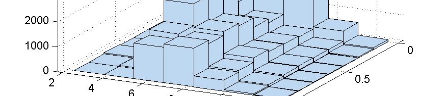
86 Figure 5.1: ROA and Employment Size (Data) Figure 5.2: ROA and Employment Size (Model) Figure 5.3: Leverage and Employment Size (Data) Figure 5.4: Leverage and Employment Size (Model) Figure 5.5: Leverage and ROA (Data) Figure 5.6: Leverage and ROA (Model) 75