Oracle Financial Services Loan Loss Forecasting and Provisioning User Guide

Transcription

1 Oracle Financial Services Loan Loss Forecasting and Provisioning User Guide Release August 2017 Part Number: E

2 Contents CONTENTS... 1 PREFACE... 6 Intended Audience... 6 Documentation Accessibility... 6 Access to Oracle Support... 6 Structure... 6 Related Information Sources INTRODUCTION UNDERSTANDING THE LLFP APPLICATION LLFP Application Process Flow LLFP CECL IFRS 9 Run Brief Overview of IFRS 9 Guidelines SEGMENTATION RUN CLASSIFICATION AND STAGE DETERMINATION Run Management Classification Rating Re-classification BASEL Re-classification Stage Determination Collective Assessment Stage Determination Run Manual Stage Reassignments HISTORICAL AVERAGE TRANSITION MATRIX Populating the Parameter Table Source Data for Historical Average Transition Matrix Historical Movement Matrix Computation Average Transition Matrix Computation HISTORICAL LOSS RATE Populating the Parameter Table Source Data for Historical Average Transition Matrix Historical Loss Rate Computation

3 7 CALCULATION OF EFFECTIVE INTEREST RATE (EIR) Overview Computation of EIR If EIR is provided as a Download EIR Computed within the Application Prerequisites for the Calculation of EIR Calculation of the EIR Value Net Present Value (NPV) of Cash Flows for Modification Gain/ Loss EIR Preferences Access EIR Preferences EIR Processing Origination Date Cash-flow Process As-Of-Date Cash-flow Process Batches to Compute EIR PROBABILITY TO DEFAULT MODELLING PD Modelling Transition Matrix Definitions Economic Scenarios PD Model Process PD Model Execution Parameters Probability to Default (PD) Term Structure PD Term Structure through Staging PD Term Structure through Seeded PD Models Movement of Data from Staging or PD Output Table to Processing Tables Interpolation of PD Values to Buckets EXPECTED CREDIT LOSS (ALLOWANCE AND PROVISION) CALCULATION IN IFRS Methodologies and ECL Calculation Methodology Selection Cash Flow Method Forward Exposure Provision Matrix Specific Provision Roll Rate Calculation of 12 Month and Lifetime ECL Irrespective of the Stage Calculation of Allowance and Provision Allowance and Provision Calculation

4 9.4 Impairment Gain or Loss Calculation Collective Assessment for ECL Run Cohort Formation for ECL Run Loss Given Default (LGD) Term Structure Obtaining LGD Data in Staging Movement of LGD Data into Processing Processing LGD Data as Required for ECL Calculation Using LGD data for ECL calculation Collective Assessment CURRENT EXPECTED CREDIT LOSS (CECL) CALCULATION FOR FASB'S CECL GUIDELINE CECL Run Management Methodologies and CECL Calculation Methodology Selection Cash Flow Method Forward Exposure Provision Matrix Specific Provision Roll Rate Calculation of Allowance and Provision Allowance and Provision Calculation Impairment Gain or Loss Calculation Loss Given Default (LGD) Term Structure Obtaining LGD Data in Staging Movement of LGD Data into Processing Processing LGD Data as Required for CECL Calculation Using LGD data for CECL calculation Troubled Debt Restructured (TDR) Reserve Computation and Adjustment RECONCILIATION Process Flow Access Reconciliation Module Search for an Existing Definition Add a Reconciliation Definition Execute Reconciliation Reconciliation Process AGGREGATE REPORTING TABLES

5 Multi Dimension Aggregate Table for Expected Credit Loss Results Segment (Portfolio) Level Aggregate Table for Expected Credit Loss Results Multi Dimension Aggregate Table for ECL Reconciliation Results Multi Dimension Aggregate Table for Roll Forward Reports EFFECTIVE INTEREST RATE (EIR) BASED INTEREST ADJUSTMENTS Overview Process Movement of Data into Processing Area Identify and Obtain Information from Last Accrual Date Transaction Level Data Population Transaction Level Processing Aggregation Account Level and Adjustment Computation ACCOUNTING ENABLEMENT RESERVE ADJUSTMENT COMPUTATION Overview Reserve Factor Definition and Reserve Adjustment Computation Process Reserve Type Access Reserve Factor Definition Section Create Reserve Factor Definition View Reserve Factor Definition Copy Reserve Factor Definition Period Specific Reserve Factor Segment Mapping Process Access Reserve Factor Segment Mapping Section Create Reserve Factor Segment Mapping Edit Reserve Factor -Segment Mapping View Reserve Factor Mapping Approve/Reject Reserve Factor Segment Mapping Execution of Reserve Factor-Segment Definition for a Specific CECL Run Computation of Required Reserve OTHER FEATURES Loss Forecasting PREPARING FOR EXECUTION Important Metadata Definition Setting Up Application Preferences Table EXECUTION

6 18.1 Data Quality Framework Run Management Run Execution from Command Line Manual Stage/Classification Reassignments Access the Maker/Checker Stage and Classification Reassignment Module Maker Stage and Classification Reassignment Process Checker - Stage and Classification Reassignment Approval/Rejection Process Legal Entity based Security for Data and Metadata Folder/Segment based Security Run Management Screen Stage Reassignment Screens LOAN LOSS FORECASTING AND PROVISIONING REPORTS IFRS IFRS 9 Stage Determination IFRS 9 Expected Credit Loss Disclosure Reports RESOLUTION OF LLFP IMPLEMENTATION ISSUES Web Service call for provision calculation Architecture Pre requisite LLFP Web Service Call Functionality ANNEXURE A: UNDERSTANDING KEY TERMS AND CONCEPTS ANNEXURE B: THINGS TO REMEMBER ANNEXURE C: FREQUENTLY ASKED QUESTIONS ANNEXURE D: PRODUCT TYPE MAPPING ANNEXURE E: DATA FLOW ANNEXURE F: GENERATING DOWNLOAD SPECIFICATION ACRONYMS AND GLOSSARY TERMS DISCLAIMER

7 Preface Intended Audience Welcome to Release of the Oracle Financial Services Loan Loss Forecasting and Provisioning (OFS LLFP) User Guide. This guide is intended for: Technical Analyst: This user ensures that the data is populated in the relevant tables as per the specifications, executes, schedules and monitors the execution of Runs as batches. Business Analyst: This user reviews the functional requirements and information sources, like reports. Data Analyst: This user would be involved with cleaning, validation and importing of data into the OFSAA Download Specification Format. Administrator: The Administrator maintains user accounts and roles, archives data, loads data feeds, and so on. The administrator would control the access rights of users. Documentation Accessibility For information about Oracle's commitment to accessibility, visit the Oracle Accessibility Program website at Access to Oracle Support Structure Oracle customers have access to electronic support through My Oracle Support. For information, visit or visit if you are hearing impaired. 1. Introduction 2. Understanding the LLFP Application 3. Segmentation Run 4. Classification and Stage Determination 5. Historical Average Transition Matrix 6. Historical Loss Rate 7. Calculation of Effective Interest Rate (EIR) 8. Probability to Default Modelling 9. Expected Credit Loss (Allowance and Provision) Calculation in IFRS Current Expected Credit Loss (CECL) Calculation for FASB's CECL Guideline 6

8 11. Reconciliation 12. Aggregate Reporting Tables 13. Effective Interest Rate (EIR) Based Interest Adjustments 14. Accounting Enablement 15. Other Features 16. Preparing for Execution 17. Execution 18. Loan Loss Forecasting and Provisioning Reports 19. Resolution of LLFP Implementation Issues Related Information Sources Oracle Financial Services International Financial Reporting Standards Application Pack Installation Guide 7

9 1 Introduction Oracle Financial Services Loan Loss Provisioning and Forecasting (LLFP) is designed to aid institutions in calculating the provision or allowance for exposures as per IFRS 9. Proposed guidelines want institutions to estimate the future loss based on forward looking factors and make provisions accordingly. Thus, the LLFP Application calculates expected loss. The International Accounting Standards Board (IASB) had published standards (IFRS 9) on calculation of loan losses and its subsequent provisioning. IFRS 9 was published in 2014 and is effective from the year It has 3 phases within: IFRS 9 (Phase I): Classification and Measurement IFRS 9 (Phase II) Impairment IFRS 9: Phase III: Hedge Accounting For more information refer, "IFRS 9 Financial Instruments" guidelines published by IASB in July Similarly, Financial Accounting Standards Board (FASB) - the US based standard setting board, which applies to organizations within USA, had come out with its own set of guidelines for loss reserve computation and provisioning, in 2016, termed CECL - Current Expected Credit Loss and the same is effective starting December

10 2 Understanding the LLFP Application The main objective of this chapter is to get familiarized with the various functions of Oracle Financial Services Loan Loss Forecasting and Provisioning, through the process flow. The logical order, in which the LLFP application functionalities are executed, helps in understanding, executing, and maintaining data in the LLFP Application. 2.1 LLFP Application Process Flow The following diagram depicts the process flow of OFS LLFP application: LLFP Data Load Segmentation Run Transition Matrix Run Loss Rate Computation Run Classification & Stage Determination Run EIR Computation Run ECL Computation Run Interest Adjustment Run CECL NOTE: This process flow diagram highlights only the key features and does not depict the entire product features. 2.2 IFRS 9 Run During financial crisis, the delayed recognition of credit losses on loans and other financial instruments are considered as a weakness in view of the existing accounting standards. Specifically, the existing model in IAS 39 (an incurred loss model) delays the recognition of credit losses until there is evidence of a trigger event. Post the crisis, the International body for accounting standards (IASB) saw the need to be proactive in recognizing the losses. Hence, IASB has issued a fresh set of guidelines for Financial Instruments - IFRS 9 related to three areas. Impairment is one of the phases / areas covered by the IFRS 9 guide lines to handle expected credit losses. The expected credit loss guidelines of IFRS 9 are more proactive and forward looking in terms of loss recognition. To be compliant to the IFRS 9 guidelines, OFSAA has upgraded its existing Loan Loss Forecasting and Provisioning application. The IFRS 9 Run includes the following Processes: Stage Determination Manual Reassignment (Optional) Expected Credit Loss Calculation Segmentation Run: In LLFP, Segmentation Run refers to the process of grouping together accounts into a Portfolio for further processing. Financial institutions generally process accounts 9

11 that have similar risk characteristics and profile together as if there were a single block/record, such as Credit Cards. Segmentation provides volume efficiency as opposed to processing records individually. Transition Matrix Run: Through a sequence of UIs, the Transition matrix user can manually feed in Probability of Default (PD) values to be later consumed in the Run apart from application s built in capability to compute historical PD values based on Credit Rating/DPD transitions over a period of time. Loss Rate Computation Run: this run computes PD value basis Roll Rate Methodology built in the application. Classification and Stage Determination Run: The Stage Determination Run starts with data population to obtain the data required for Classification, Stage Determination, and ECL computation. The non-standard/external data formats are now reclassified to standard/internal data formats. The final sub process is to assign a stage at an account level granularity (either through Individual or collective basis) based on the data provided and rules configured. After this the reclassification sub process is executed to convert non-standard/external data formats to standard/internal data formats. The next process is to conduct the Business model and Cash Flow Characteristics (SPPI) test to identify the classification for each instrument / account. The final stage is to evaluate the change in credit risk and macro economic factors to determine the stage at an account level granularity with the stage determination sub-process. Upon successful execution of the stage determination run, the application provides an option for the manual reclassification of the stages assigned to accounts, based on various parameters. Manual Reassignment: This optional step enables the financial institutions to override the outcome of the Stage Determination Run and reassign the stage. This process goes through a Maker- Checker workflow with an audit trail. It caters to any judgmental or qualitative factors that needs to be considered plus any reputable presumptions. ECL Run: The ECL Calculation Run begins with the Methodology Selection sub process to assign a specific calculation methodology for each of the accounts processed by the application. The selection of methods is based on specific factors that are taken into consideration by the application. Post methodology selection, the application then calculates the Expected Credit Loss, again at an account level granularity (either through Individual or collective basis), based on the approach as per the method selected. The ECL values are also calculated for off-balance sheet accounts, undrawn portion, POCI accounts, and so on. Interest Adjustment Run: IFRS9 requires interest income recognition at Effective Interest Rate. Adjustment value will be posted after factoring in the contract interest amount Brief Overview of IFRS 9 Guidelines The methodologies to calculate the Expected Credit Loss for different instruments under various Credit Risk scenarios are provided by the IFRS 9 guidelines. Following are those instruments that fall under the scope of IFRS 9 Impairment standards: Financial Assets measured using Amortized cost or Fair Value through OCI 10

12 Lease Receivables and Trade Receivables Contract Assets, Loan Commitments and Financial Guarantees The different methodologies highlighted by the standards, are: General Approach Simplified Approach Approach for Purchased or Originated Credit Impaired (POCI) Accounts General Approach The General Approach is for all instruments that are within the scope of IFRS 9 except for Lease Receivables, Trade Receivables, Loan Commitments, Contract Assets, and any other instruments that are Purchased or Originated Credit Impaired. Under this approach, the standard requires the entity to measure the significance of Increase in Credit Risk of the instrument, since its initial recognition. Based on the outcome, the entity provides for a 12 Month Expected Credit Loss or a Lifetime Expected Credit Loss. If the entity decides that there is No Significant Increase in Credit risk, then the Allowance is equal to the 12 Month Expected Credit Loss. If the entity decides that there is a Significant increase in Credit Risk, then the Allowance is equal to the Lifetime Expected Credit Loss. The standard also provides detailed guidance on the factors to be considered to decide the significance of Increase in credit risk of an Instrument. In case, the instrument becomes impaired, the Allowance is equal to the difference between the Gross Carrying Amount and the present value of the expected cash flows Simplified Approach IFRS 9 standards state that, for certain specific instruments, it is not essential to determine the significance of increase in Credit risk. Instead, an Allowance equal to the lifetime Expected Credit Loss can be directly provided. The instruments in scope of the simplified approach are: Lease Receivables Trade Receivables, Loan Commitments, and Contract Assets without significant financing component Trade Receivables, Loan Commitments, and Contract Assets with significant financing component and the entity chooses to follow the simplified approach. NOTE: For Trade Receivables, Loan Commitments, and Contract Assets with significant financing component, the entity has the option to choose either the general approach or the simplified approach. 11

13 Approach for Purchased or Originated Credit Impaired (POCI) Accounts The Allowance calculation of POCI accounts under this approach requires the calculation of the Lifetime Expected credit loss for each account, using the Credit Impaired EIR as the discount rate. The allowance is the cumulative change in the lifetime expected credit loss for the account since date of initial recognition Determining Significance of Increase in Credit Risk The standard also provides a view point on the various factors that an organization should take into account to determine if a particular instrument (that is not Purchased or Originated Credit impaired) has seen a significant increase in credit risk or not. Some of the factors suggested by the standard are: Internal Price indicators of Credit Risk Attributes of Financial Instruments such as Covenants, Collateral, and so on. Credit Spread, Credit Default Swaps, Fair Value less than Amortized Cost External Credit Rating Internal Credit Rating Forecast of Financial Conditions Forecast of Economic Conditions Forecast of Business Conditions Increased Credit Risk on other financial instruments of the borrower Adverse change in the Regulatory, Technology environment of the borrower Change in value of the collateral Change in quality of guarantee Support from Parent organization Expected changes in the Loan documentation Expected changes in the performance and behavior of the borrower Past due information Qualitative and non-statistical Factors 12

14 3 Segmentation Run Segmentation Run of LLFP is one of the foremost runs that need to be executed during the process of computing various parameters required under IFRS 9. However, the use of segments (execution of the Segmentation run) is not mandatory. If you do not want to use features that require segments (for example, Historical Transition Matrix, PD Model, and so on). Segmentation is the process of grouping accounts into homogenous clusters using various dimensions as parameters. Segments or Portfolios help in simplifying the process of treating/evaluating accounts by treating accounts belonging to one homogenous group in the same manner. The Segmentation Run of LLFP can be used to create such Segments/Portfolios, wherein every account is mapped to a specific Segment. The first step in the Segmentation process is to create a Segment Type and the master list of Segments that you wants to map each of the accounts to, using the AMHM screens. The standard product has a seeded Segment Type IFRS9 ECL and corresponding Segments. You can choose to use the existing Segments or create a new Segment type and corresponding child Segments. Once the master list of Segments are available, the second step is to configure Rules that assign a Segment to an account taking into consideration various dimensions, using the flexible (configurable) Run Rules Framework. The standard product considers two dimensions to assign a Segment to an account. These are Product Type and Customer Type. As required, more Dimensions can be considered by reconfiguring the dataset and the Rule, such as Industry, Region, Branch, Country, and so on. The output of LLFP s Segmentation Run is stored in a specific table where for any given date only one set of Account-Segment mapping, the final one, is stored. This mapping is then taken into account for further processing in both the LLFP application as well as OFSAA s Hedge Management application. Segmentation is mandatory for the functioning of following features: Historical Transition Matrix Historical Loss Rates Inbuilt PD Model ECL Computation using Roll Rate Methodology 13

15 4 Classification and Stage Determination 4.1 Run Management OFS LLFP application supports two sequential runs (Stage Determination and Allowance Calculation) that are seeded within the application to support the Expected Credit Loss (Allowance and Provision) calculation as per the IFRS 9 guidelines. The Stage Determination run starts off with the data population sub processes to obtain the data required for both Stage Determination. After this the reclassification sub process is executed to convert nonstandard/external data formats to standard/internal data formats. The final stage is to evaluate the change in credit risk and macro economic factors to determine the stage at an account level granularity with the stage determination sub-process. Upon successful execution of the stage determination run, the application provides an option for the manual re-classification of the stages assigned to accounts, based on various parameters. Upon completion of manual reclassification of stages, the application obtains the additional data required for ECL calculation. The Cash Flow and Forward Exposure sub processes along with the Probability of Default calculation is performed and the ECL amount is calculated. Separate processes are applicable for the Provision Matrix and Specific provision methods. The application also displays the execution status of the Run through the UI. For more details, refer Run Management section. Upon successful execution, the outputs including but not limited to, Expected Credit Loss, Allowance, Provision, Effective interest rate and so on are available for reporting Classification Financial instruments are required to be classified into three categories and thereby accounted as suggested in the Phase 1 section of the IFRS 9 guidelines. The three categories are the following: Amortized Cost (AMRTCOST) Fair Value through Other Comprehensive Income (FVOCI) Fair Value through Profit and Loss (FVTPL) Financial assets should undergo Business Model test (BM) and Cash Flow Characteristics test (SPPI) and Financial Liabilities should undergo the Business Model Test for classifying in the afore mentioned categories Business Model Test The Business Model Test is conducted at an aggregated level. This test allows the banks to classify instruments into any of the sub categories of business model such as Held to Collect (Assets), Held to Collect and Sell (Assets), Held to Sell (Assets and Liabilities), Held to Maturity (Liabilities), and Available for Sale (Liabilities). 14

16 To conduct the Business Model Test, various dimensions are considered to assign a business model. You can create Rules that are executed in a specific order and that helps in the categorization. The application is seeded with certain Rules which can be modified or removed. The Rules around Business Model Test enable banks to design a hierarchy based Holding Type assessment, that is the Rules help banks to classify its accounts into any one of the holding types, such as Held to Collect, Held to Sell or Held to Collect and Sell. Banks are able to configure Rules based on various available Hierarchies or a combination of Hierarchies. For example Portfolio, Customer Type, Product, Branch, Industry, Country, and Line of Business, and so on. The standard product consists of the following rules: Source Dimensions Product, Customer Type Product, Capital Exposure Flag Product, Exposure for Sale Indicator Target Dimension Holding Type Holding Type Holding Type Cash Flow Characteristics (SPPI) Test IFRS 9 requires all financial instruments to be tested for their cash flow characteristics before being classified into any of the three accounting classifications. This test is conducted at the instrument level. To pass the cash flow characteristics or the Solely Payments of Principal and Interest (SPPI) test, an entity needs to prove that the contractual cash flows received from an instrument are Solely Payments of Principal and Interest on the principal amount outstanding. To conduct the Cash Flow Characteristics Test, various dimensions are considered. However, more importantly, the contract level characteristics are taken into consideration with the help of certain flags, parameters, values, and so on. This defines the instrument in detail. The application picks the dimension based Rules to assign the SPPI flag as YES. Primarily, the SPPI flag is assigned based on the broad knowledge on the Portfolio, Product, or Product type. Once the SPPI flags are assigned based on a given set of dimensions, further evaluation is conducted for those accounts with SPPI flag as YES. The Rules related to SPPI test enable the bank to evaluate every instrument/account to check if the contractual cash flows received from an instrument are Solely Payments of Principal and Interest on the principal amount outstanding or SPPI. The initial set of Rules allow the user/bank to define if a product /portfolio may potentially pass the SPPI test, at an aggregated level (that is, the hierarchy at which the Rule is defined). All the subsequent Rules verify the characteristics of an instrument to check if it caters to the SPPI requirements. The standard product consists of the following Rules: Source Dimensions Target Dimension 15

17 Source Dimensions Product Behavior Type = Devolvement and Recovery If SPPI= Y, Fixed, Interest Rate<=0% If SPPI= Y, Floating Rate, Float Spread<=0% If SPPI= Y, Embedded Options Flag = Y If SPPI= Y, Securitized Flag= Y If SPPI= Y, Employee Account = Y If SPPI= Y, Sub Prime Flag= Y If SPPI= Y, Payment Pattern <any specific pattern> If SPPI= Y, Benchmark Currency<>Instrument currency Target Dimension SPPI SPPI = N SPPI = N SPPI = N SPPI = N SPPI = N SPPI = N SPPI = N SPPI = N SPPI = N NOTE: You can configure/reconfigure the given Rules and also add/remove Rules as per the requirement Accounting Classification based on Business Model and SPPI Once Business Model test or Cash Flow Characteristics test is performed, the classification method needs to be assigned, depending on the outcome of the test. As the first step, accounts that have been assigned the classification through staging or based on election retain that classification. For accounts, where the classification is null, the following process assigns the classification: Business Model SPPI Test Classification Held to Collect Y AMRTCOST Held to Collect and Sell Y FVOCI Held to Sell Y FVTPL Held to Maturity Y AMRTCOST Available for Sale Y FVTPL Held to Collect N FVTPL Held to Collect and Sell N FVTPL Held to Sell N FVTPL Held to Maturity N AMRTCOST 16

18 Business Model SPPI Test Classification Available for Sale N FVTPL The final process is to optionally select the accounts to be classified under FVTPL or FVOCI. This is done based on the following Rules: 1. Fair Value option: If fair value flag is Y, then Classification = FVTPL 2. Equity Instruments: For Instrument Type = Equities and Business Model = Held to Collect, then Classification = FVOCI NOTE: If the Classifications for all the accounts are provided as downloads, then the application need not process the same. In such cases, all the Classification related Processes have to be removed from the Stage Determination and Classification Run. OFS LLFP application does not support providing Classification as download and processing Classification partially by the application Rating Re-classification In this sub process, the application re-classifies the external ratings to internal ratings. This is necessary because the wide variety and range of external ratings from various sources have to be mapped to the user s limited set of the internal rating, for ease of processing and comparisons BASEL Re-classification Basel reclassification Rule is used to map the bank s customer type and product type to Basel Customer Type and Basel Product Type respectively. Product types, Customer types, and Asset classes are reclassified to standard values for further processing. This is performed with the aid of the following reclassification Rules: Basel Product Type Re-classification Basel Customer Type Re-classification Basel Asset Class Re-classification Basel Product Type Re-classification In Basel Product Type Re-classification, the bank s product type is mapped to the Basel product Type Basel Customer Type Re-classification In Basel Customer Type Re-classification, the bank s customer type is mapped to the Basel Customer Type. 17

19 Basel Asset Class Re-classification In Basel Asset Class Re-classification, the asset classes are standardized for further processing Stage Determination Stage Determination is a sub process in the Stage Determination run. The IFRS 9 guidelines require each account to be classified into three different stages on every reporting date, based on the significance of increase in Credit Risk since initial recognition. The guidelines mandate the calculation of a 12 Month or Lifetime Expected Credit Loss for an account, depending upon the stage in which an account (instrument) has been classified into. The LLFP application supports the Stage Determination requirements of the IFRS 9 guidelines by considering the following factors to determine the Significance of Increase in Credit Risk, thereby deciding the stage in which a particular account is classified into: Rating for all customer types other than Retail (Long term or Short term) Delinquency Days-past-due (DPD) and LTV for Retail customers Industry Country Devolvement status New account Restructured status Impaired/Default Status The stage determination rules based on the IFRS 9 Rules are created using any one of the parameters provided above and each of these rules are available in the out of the box product. The rules are pre-built and easily reconfigurable based on the internal risk policy of the bank or based on the regulator s directions. The application allows the user to create new rules from the data available in the model, modify the existing rules, delete specific rules and reorder the entire set of rules. Collective Assessment: The ECL run can also determine the stage, collectively (at an aggregated level). For more information, refer Collective Assessment section. Rating: This rule is applicable for wholesale type of accounts. Depending upon the Rating on the Date of Initial Recognition and the Rating on the Current reporting date, the accounts are classified into one of the three stages. Rating as of Initial Recognition is obtained as a download and is reclassified to the Internal Rating. The user can configure what number of notches degraded should be considered as significant increase of Credit Risk Delinquency Past Due days: This rule is applicable for all retail type of accounts. 18

20 LTV: This rule is applicable for specific product types such as Secured Lending and Residential Mortgage Exposure. This rule requires the pre-calculation of the LTV Change. Exposure LTV Ratio is obtained as a download. Exposure LTV Ratio on Date of Initial Recognition is obtained as a download. If the LTV change is greater than the application, it can classify such accounts from Stage 1 to 2. This value can be customized by the customer. New Account: This rule is applicable for all accounts. It ensures that the new accounts are classified as Stage 1, immaterial of its rating or DPD/LTV values as of the current reporting date. Devolvement Status: This rule is applicable only for Loans and Guarantees (Direct Credit Substitutes). The rule classifies all devolved accounts into stage 2. Industry: This rule is common for both the retail as well as wholesale type of accounts. The rule can be customized for each run to reflect the economic scenarios at that instance. Country: This rule is common for both the retail as well as wholesale type of accounts. The rule can be customized for each run to reflect the economic scenarios at that instance. Simplified: This rule is to ensure that certain product types are directly classified as Stage 2 by the application. Restructured (Renegotiated or Modified): This rule ensures that renegotiated or modified accounts are retained in Stage 2 for a certain period of time (Observatory Period) beyond the date of modification. This time is calculated upfront by the pre-calculation process. The application checks if the time since date of Modification (Current date Date of Modification) is within the Observatory period. All modified accounts that are classified into stage 1 and 2 by earlier rules and within this time period, will be bucketed into Stage 2. Any account classified into Stage 3 by earlier rules will be retained as Stage 3. The user can configure the duration of the Observatory period either as an absolute value or a percentage value. 12 Month PD: This Rule compares the 12 month PD as of Origination Date with respect to current 12 month PD and migrates the account to Stage 2, if the difference is greater than the threshold value of 20 percentage points. However, this Rule can be configured to change the threshold value for as per your requirements. This Rule can also be modified to compare the PDs on relative basis instead of absolute basis.. Impaired: This rule ensures that all impaired accounts are classified into Stage 3. Default: This rule ensures that all defaulted accounts are classified into Stage 3 Stage Migration Check: This rule is to ensure that there is no movement of accounts from Stage 3 to Stage 1 between two consecutive reporting dates. NOTE: The Rules stated here are part of out of the box application. New Rules can be added to this list and the existing Rules can be modified or removed, depending on the Banks discrete Risk policy. While classification is done for all instruments, the Stage and ECL Computation are done only for Asset classes and certain off balance sheet instruments. This is a configurable idea wherein you may select the list of products that have to be 19

21 considered for Stage Determination and ECL computation. This is achieved through a Rule Collective Assessment Stage Determination Run The Collective Assessment feature of the IFRS 9 Run of LLFP application enables you to form Cohorts (that is, group a set of accounts) based on various parameters/dimensions such that, accounts with similar characteristics are grouped together and treated uniformly as a single account, while determining the stage as well as computing the Expected Credit Loss (ECL) values Cohort Formation for Stage Determination Run The Collective assessment feature is part of the IFRS 9 Stage Determination Run and it addresses the following two major aspects: Determine the stage of accounts with similar (Risk) characteristics in a similar manner Improvement in performance by reducing the total number of records to be treated The application uses the following steps during the Stage determination process, specifically related to collective assessment: A configurable rule that defines the dimensions/parameters deciding the set of accounts that are allowed to be processed, collectively. Cohort formation (grouping of accounts) based on a given set of dimensions. Assigning/calculating Cohort level values based on the account level values, which are part of the Cohort. Determine the Stage for Cohorts Reassign the Cohort s stage back to individual accounts that are part of the Cohort. These steps are detailed in the forthcoming sections: Dimensions/Parameters Deciding the Type of Accounts that are allowed to be Processed Collectively This process has been approached in the following two steps: Parameters/dimensions that mandatorily filter out specific accounts from collective assessment. Accounts matching the following parameters are eligible for collective assessment. Account should not have been restructured Account should not be impaired or defaulted Account should not be a POCI account Account should not have been devolved 20

22 Account should not have been classified as stage three in the previous reporting date NOTE: These are mandatory filters that cannot be changed. Dimensions that decides the set of accounts enabled for collective assessment Using the Run Rule framework, the application enables you to define the dimensions that determine which set of accounts are allowed to be treated collectively. The Rule is flexible enough to allow you to include new dimensions, remove existing ones, and so on. In the out of the box product, the default dimensions are: Basel Customer Type Basel Product Type Dimensions based on which Accounts are grouped Once the accounts that are eligible for collective assessment are decided, the next step is to decide the parameters based on which the groups are formed. LLFP forms Cohorts based on the following dimensions: Basel Customer Type Basel Product Type Country Industry In addition to the preceding dimensions, For non-retail customer type, the following two dimensions are also considered for cohort formation: Rating (counterparty or issuer) on Initial Recognition and Rating (counterparty or issuer) as of Current date For retail customer type, the following dimension is also considered for cohort formation: Delinquency past due days band Assigning Values to Cohorts Once the Cohorts are formed, they are treated as individual accounts. The next step is to assign representative values to the parameters of these Cohorts based on the values of accounts that are part of the Cohort. The following table highlights, how the representative values are computed for the given parameters of a Cohort: FISD Columns Collective Individual Flag Exposure Default Status Flag Values "G" "N" 21

23 LTV Flag Account Sequence Number Calculated post cohorts automatically Cohort ID Account SKey -1 Basel Customer Type SKey Basel Product Type SKey Counterparty Rating DOIR SKey Counterparty Rating SKey Country SKey Delinquency Bank SKey Development Status CD Customer Industry SKey Issuer Rating DOIR SKey Issuer Rating SKey LTV Currency Ratio LTV DOIR Ratio MIS Date SKey Run SKey As per Cohort As per Cohort As per Cohort As per Cohort As per Cohort As per Cohort As per Cohort As per Cohort As per Cohort As per Cohort Average Average As per Run As per Run Stage Determination of Cohorts For facilitating the Stage Determination process of the Cohorts, the application s Stage Determination Rule has been reconfigured to work either on Individual accounts not part of Cohorts or on Cohorts. NOTE: The Stage Determination Rules do not process Individual accounts that are part of Cohorts. Reassigning the Stages Assigned to Cohorts back to Individual Accounts Once the stage is determined for the Cohorts, the same is assigned back to individual accounts. Audit Trail After this, the Cohort related records are removed from the IFRS Stage Determination fact table and moved to a new table for audit purposes. 22

24 4.1.6 Manual Stage Reassignments The Manual Stage Reassignments/Overrides UI enables the user to manually update any stage that was assigned to every account by the application using the Stage Determination rules. The stage is assigned through the Stage Determination run. For more details on Stage Determination, refer to Stage Determination Run section. The manual reassignment of the stage determination involves two steps: Manual reassignment step Approval process The users who have the Maker (manual reassignment step) privileges can update the rating using the Stage Reassignment section of the Maker Stage Reassignment module. The approval/rejection process is performed by the user who has the Checker privileges. The checker can use the Stage Reassignment section of the Checker Stage Reassignment module to approve/reject the reassignments done by the user who had the Maker privileges. To know more about the Manual Reassignment Process, refer to Manual Stage/Classification Reassignments section. NOTE: The Preferred Segment Type Code should be updated in the Preference table for the successful execution of the Run. If you do not want to use Segments as a Dimension, the related Processes must be removed. 23

25 5 Historical Average Transition Matrix Historical Transition Matrix is generated using long term averages and can be based on rating scales or DPD bands. The last column of this matrix is the default probability also called the long term default frequency. The Historical Transition Matrix Run is used to compute the average Transition Matrix for various portfolios / segments based on the historical data available within the application. The Run can be segregated into two functional steps: 1. Transpose the historical data between any two dates into a movement matrix. 2. Look up the movement matrix across multiple dates to compute the Average Transition Matrix. 5.1 Populating the Parameter Table Generation of a Transition Matrix requires certain parameters to be defined; this is done with the help of Rules that populates the values in a specific Param table. The parameters are defined at segment / portfolio level. The parameters that are required to be defined are the following: EIR Computation Flag: Identifies the portfolios/segments for which Transition matrices have to be created. Transition Matrix Type: Defines whether the matrix should be based on Rating (R) or Delinquency Past Due Days Band / DPD Bands (D). Transition Matrix Frequency: Indicates the frequency of the matrix as Annual (Y), Semi Annual / Half Yearly (H), Quarterly (Q), and Monthly (M). Transition Matrix Basis: Indicates if the computation happens on the basis of Number of Accounts (N) or Outstanding Amount (O). The Rules that populate the Param table are configurable based on the requirements of the customer (preferably as a onetime activity). NOTE: Segmentation (Portfolios) is a mandatory prerequisite for the computation of Historical Transition Matrix. 5.2 Source Data for Historical Average Transition Matrix The source data for both Historical Average Transition Matrix and Historical Loss Rate computation is the Common Account Summary Fact table, where data across each MIS Date is available at an account level granularity. The FCAS table has sufficient information across multiple dimensions that help map each account to a Rating or Delinquency Past Due Band and the various segments under which the accounts fall. 24

26 5.3 Historical Movement Matrix Computation The first step in the Average Transition Matrix computation process is to compute the movement matrix between the MIS Date and the previous Date. Once the two dates are arrived at, the accounts under each valid segment are grouped based on the combination of the Previous and Current Rating or DPD Band. Once the accounts are grouped, the movement amounts/values are computed between any two Ratings or DPD bands. The previous date is inferred based on the Frequency of the Matrix as per the assignment made in the Param table for the given Segment. Transition Matrices are generated only for Segments with TM Compute flag marked as Y in the Param table. The Rating or DPD basis is decided per the values assigned in the Param table for the given segment. The basis of computation - Number of Accounts or the Outstanding Amount of the Account is decided per the values assigned in the Param table for the given segment. 5.4 Average Transition Matrix Computation The second step in the process is to compute the Average Transition Matrix, based on the Rating / DPD band movements computed across historical dates (in the previous step). The number of periods to look back is decided based on the Preferences set in the LLFP Preference table, based on which the outstanding amounts or number of accounts are summed up for the computation purpose. In order to compute the Transition Rates, the total migration value (Number of accounts or Outstanding amount) between any two Ratings or DPD bands is divided by the total value (Number of Accounts or Outstanding Amount) on the base Rating or DPD Band. The results (Transition Matrices) across segments are then stored in the Transition Matrix Master and Transition Matrix Details tables. NOTE: During the initial Run, historical data will not be available for computation. You need to ensure that historical data is populated manually before executing the Historical Matrix Run. OFS LLFP application stores all the required data from the initial Run onwards. The duration of required historical data is dependent on the value provided in the Transition Matrix Historical Data Cap and Transition Matrix Historical Data Cap Unit columns of the Application Preferences table. If you update the Transition Matrix frequencies that was previously set in the application, you will have to re-execute all the pre-executed Runs (for the duration mentioned in the Application Preference table). Historical data needs to be populated to the columns of the table (FSI_LLFP_AVG_MOVEMENT_MTX) as tabulated in the List of Columns for Historical Data One Time Load spreadsheet, available in the following MOS document:

27 6 Historical Loss Rate The Historical Loss Rate Run is used to compute the loss rates for various Portfolios / Segments based on the historical data available within the application. 6.1 Populating the Parameter Table Computation of Historical Loss Rate requires certain parameters to be defined. This is done with the help of Rules that populates the values in a specific Param table. The parameters are defined at a Segment / Portfolio level. The parameters that are required to be defined are the following: EIR Computation Flag: Identifies the Portfolios/Segments for which Transition matrices have to be created. Transition Matrix Type: Defines whether the matrix should be based on Rating (R) or Delinquency Past Due Days Band / DPD Bands (D). Transition Matrix Frequency: Indicates the frequency of the matrix as Annual (Y), Semi Annual / Half Yearly (H), Quarterly (Q), and Monthly (M). Transition Matrix Basis: Indicates if the computation happens on the basis of Number of Accounts (N) or Outstanding Amount (O). The Rules that populate the Param table are configurable based on the requirements of the customer (preferably as a onetime activity). NOTE: Segmentation (Portfolios) are a mandatory prerequisite for the computation of Historical Transition Matrix 6.2 Source Data for Historical Average Transition Matrix The source data for both Historical Average Transition Matrix and Historical Loss Rate computation is the Common Account Summary Fact table, where data across each MIS Date is available at an account level granularity. The FCAS table has sufficient information across multiple dimensions that help map each account to a Rating or Delinquency Past Due Band and the various Segments under which the accounts fall. 6.3 Historical Loss Rate Computation The first processing step in the Historical Loss Rate Computation process is to group all the accounts based on the Default Grade Rating or the Default DPD Band for the given date. Once the accounts are grouped, the total outstanding, total recovery, and total write-off amounts are summed up across these accounts. This step is done only for the given MIS Date. NOTE: Only the accounts in the default grade are considered. The second step in the process is to compute the Loss Rate for the given MIS Date using the following formulae: 26

28 Loss Rate (t) = [Write-offs (t) Recoveries (t) ] / Outstanding (t-1) These loss rates are then used for the Average 12 month and Life time Gross Loss Rate computation within the Roll Rate methodology. NOTE: During the initial Run, historical data will not be available for computation. You need to ensure that historical data is populated manually before executing the Historical Loss Rate Run. OFS LLFP application stores all the required data from the initial Run onwards. The duration of required historical data is dependent on the value provided in the Loss Rate Historical Data Cap and Loss Rate Historical Data Cap Unit columns of the Application Preferences table. If you update the Loss Rate frequencies that was previously set in the application, you will have to re-execute all the pre-executed Runs (for the duration mentioned in the Application Preference table). Historical data needs to be populated to the columns of the table (FSI_LLFP_HIST_LOSS_RATE) as tabulated in the List of Columns for Historical Data One Time Load spreadsheet, available in the following MOS document:

29 7 Calculation of Effective Interest Rate (EIR) 7.1 Overview IFRS 9 mandates the use of Effective Interest Rate (EIR) for the purpose of discounting to take in to account the Time value of money. The guidelines also mandate the use of Origination date EIR for Fixed rate accounts and Current date EIR for Variable rate accounts. Additionally, the guidelines require the banks to use Credit Adjusted Effective Interest Rate (CAEIR) in case of any Purchase or Originated Credit Impaired (POCI) accounts. As mentioned, for fixed rate POCI accounts, the Origination date Credit Adjusted EIR is used and for variable rate accounts Current date Credit Adjusted EIR is used. 7.2 Computation of EIR The LLFP application calculates the Effective interest Rates as applicable. The application also gives an option to provide the EIR value as a download. NOTE: EIR computation is applicable for products under ODs, Cards, Loans, Investments, Money Market instruments, Borrowing, Repo Contracts, Annuity Contracts, Term Deposits, Commitment Contracts, and Retirement Accounts. In case of Leases, the Lease rate is used as the discount rate. And for Letter of Credits and Guarantees, the discount rate is provided as a download. These rates have to be provided as download through the Account Inception Rates Stage table. Holiday Calendar is not supported for EIR Computation. Credit Adjusted EIR is not computed If EIR is provided as a Download If the value is provided as a download through the staging table Account Inception Rates Stage table, then the application populates the same into the processing area. In case of a fixed rate account, the application checks the availability of the corresponding to the given Account ID as per the account start date (MIS Date = Account Start Date). In case of a variable rate account, the application checks the availability of the EIR corresponding to the given Account ID as per the given MIS Date. NOTE: If the EIR for the required date is not available in Account Inception Rates table, then EIR on the MIS Date, which is nearest to required date is used EIR Computed within the Application The following two approaches are used to compute the EIR within the application: Cash Flows Generated by Oracle s Cash Flow Engine Cash Flows Provided as Download 28

30 Cash Flows Generated by Oracle s Cash Flow Engine In this scenario, the application requires Oracle Financial Services Asset Liability Management (OFS ALM) as a prerequisite and the user needs to populate all the relevant columns mandated by the cash flow engine. For more information, see Oracle Financial Services Asset Liability Management User Guide in Oracle Help Center Documentation Library. In addition, there are certain columns required for the purpose of computing the EIR as of Origination date, such as original deferred balances, and so on. These columns are identified in LLFP s download specifications. For more information, see Oracle Help Center Documentation Library. Execution: You must use the EIR Preference screen where you can identify the process created in the OFS ALM application to generate the cash flows (As-of-Date or Origination date). Once the process(es) are identified, the relevant Batches needs to be executed to compute EIR. For more information on Batches, see Batches to Compute EIR section Cash Flows Provided as Download In this scenario, the application requires cash flows to be provided in the staging area and account related attributes to be provided in the corresponding columns in the product processors. Execution: The relevant Batches needs to be executed to compute EIR. For more information on Batches, see Batches to Compute EIR section. NOTE: When Cash Flows are provided as download, the application computes EIR solely for assets and only cash in-flows are considered EIR Calculation Flag and Checking the Availability of EIR Value (For Fixed Rate Account Origination Date EIR The EIR EIS Calculation Flag determines the need to re-calculate the Origination Date EIR. NOTE: EIR as of current date is computed every time, irrespective of the Flag. If the flag is Y in Product Processor table, application computes/re-computes Origination Date EIR value. If the flag is NULL in Product Processor table and the EIR is not available for the given account, then application computes the same Prerequisites for the Calculation of EIR The application requires the following values for calculation of EIR: If Cash Flows are given as download Cash Flows as of Origination date for fixed rate accounts and Cash Flows on As-of-Date for Variable rate accounts. If Cash Flows are to be generated by OFS ALM - Account related attributes (As required by OFS ALM s Cash Flow Engine). 29

31 Data Prerequisites for EIR Computation Key Parameters Fixed Rate Floating Rate Outstanding Original Outstanding Current Outstanding Cash Flows As of Origination Date As of given date Fees (Applicable for EIR) Original Fees (as of origination) Deferred Fees (As of current date) Premium / Discount Original Premium or Discount Deferred Premium or Discount Cost Original Cost Deferred Cost Other parameters (for example, Payment frequency, Current Rate, and so on) Detailed data requirements are mentioned separately. Constant across both NOTE: This table is only to indicate the Origination Date vs As of Date data requirements (for Origination date EIR and As of Date EIR) Calculation of the EIR Value The application first adjusts the outstanding amount with fees (specific to EIR), any premium or discount, and any cost. After this, the internal rate of return is computed using the adjusted outstanding amount and the Cash Flows Net Present Value (NPV) of Cash Flows for Modification Gain/ Loss Net Present Value (NPV) of Current Date Cash Flows are determined for both Fixed and Floating rate accounts. Then the cash flows are discounted using the EIR to compute the NPV. For Fixed rate accounts, origination date EIR is considered and for Floating rate accounts, As of Date EIR is considered. This Net Present Value of cash flows is used to compute Modification Gain / Loss. For more information, see Modification Gain / Loss section. 7.3 EIR Preferences The EIR Preferences section enables you to select processes for Effective interest Rate (EIR) calculation. EIR is calculated using both Origination Date Cash Flows and As of Date Cash Flows and the Cash Flows are discounted over the lifecycle of the financial asset. 30

32 For EIR computation, be it Origination Date or As of Date, ALM is used to the extent of generating the cash flows. Subsequent calculation of EIR is only within LLFP. Therefore, it is required to set up the required Static Deterministic Processes within ALM (ideally, these can stop with cash flow generation). After this, everything is controlled from inside LLFP. You will need to schedule/execute an LLFP- Engine this engine will internally trigger the CFE; once the CFE completes, the cash-flows are picked up and EIR is computed for each account Access EIR Preferences Once the required number of ALM processes are setup within ALM, the EIR Preferences section can be used to specify which ALM processes are used for As of Date and which are used for Origination Date. You can access EIR Preferences screen by clicking Loan Loss Forecasting and Provisioning > LLFP Maintenance > EIR Preferences link from the LHS menu of the application. The EIR Preference screen is displayed as depicted in the following figure: EIR Processing For EIR calculation, the OFS LLFP application provides you the option to select multiple processes. Various such different processes can be marked for Origination Date Cash Flows and As of Date Cash Flows. NOTE: You must ensure that the same set of account(s) is not included across multiple processes Origination Date Cash-flow Process This section details you the process of selecting processes from the list of available processes, in OFS LLFP application for Origination Date Cash Flow process Process Selection Perform the following procedure to select the required processes: 1. Click button present in the Origination Date Cash-flow Process grid. The Process Selection window is displayed. 31

33 2. Select the folder from the drop down list adjacent to the Folder field. The available processes are displayed under the Process Selection grid. For Origination Date Cash Flows, the Generate Cash Flow check box is selected by default. 3. Click to mark the required processes. You can use the Control key to mark multiple processes. 4. Click button to select the marked processes by moving those from the list of processes pane to the selected processes pane. You can also perform the following for selecting processes: Click button to select all the processes. Click button to deselect the selected processes by moving those from the selected processes pane to the list of processes pane. Click button to deselect all the processes. 5. Click button. The selected processes are saved and are displayed under the Origination Date Cashflow Process grid As-Of-Date Cash-flow Process This section details you the process of selecting processes from the list of available processes, in OFS LLFP application for As of Date Cash Flow process Process Selection Perform the following procedure to select the required processes: 1. Click button present in the As-Of-Date Cash-flow Process grid. The Process Selection window is displayed. 32

34 2. Select the folder from the drop down list adjacent to the Folder field. The available processes are displayed under the Process Selection grid. 3. Select the check box adjacent to the Generate Cash Flow field, if you want to generate Cash Flows. 4. Click to mark the required processes. You can use the Control key to mark multiple processes. 5. Click button to select the marked processes by moving those from the list of processes pane to the selected processes pane. You can also perform the following for selecting processes: Click button to select all the processes. Click button to deselect the selected processes by moving those from the selected processes pane to the list of processes pane. Click button to deselect all the processes. 6. Click button. The selected processes are saved and are displayed under the As-Of-Date Cash-flow Process grid. 7.4 Batches to Compute EIR There are the following batches, which are used in EIR calculation, for Origination Date and As of Date: Batch Name: <Infodom>_LLFP_EIR_INST_DATA_POP This Batch is for Origination Date Cash flow Generation and EIR computation. Batch Name: <Infodom>_IFRS_AOD_CF_EIR This batch is for Current Date Cash Flow Generation and EIR computation. Batch Name: <Infodom>_LLFP_CF_EIR_INST_DATA_POP This batch loads data from the product processor tables into the respective instrument tables (FSI_D_*). 33

35 For more information on configuration of ifrs-eir.ini file, refer to Oracle Financial Services International Financial Reporting Standards Application Pack Installation Guide version in OHC Documentation Library. When Cash Flows are provided as download, you need to modify the Batch parameters. To know more about these modifications, see OFS LLFP Run Chart in OHC Documentation Library. To know more about Batches and Batch Execution, see Operations chapter in Oracle Financial Services Analytical Applications Infrastructure User Guide available at OHC Documentation Library. The behavior of the IFRS EIR engine is controlled by six execution properties present in ifrseir.ini file. To know more about these properties and their functionalities, see Update the Properties of ifrs-eir.ini file section in OFS IFRS Installation Guide available at OHC Documentation Library. 34

36 8 Probability to Default Modelling 8.1 PD Modelling OFS LLFP PD Modelling accurately predicts the number of defaults by omitting optimism or conservatism. Adjustments are made on regulatory capital models to remove inherent conservatism. Estimated PDs are point-in-time. These are adjusted, where necessary, to reflect the effects of the current economic conditions. The PD estimates are recalibrated based on current representative sample on a regular basis. PD is calculated using sufficient sample size and historical loss data covers at least one full credit cycle. PD model segments consider drivers in respect of borrower risk, transaction risk, and delinquency status. The PD models are representative of the portfolio segments. The data used for calibration is consistent with the IFRS 9 default definition throughout. Techniques used to determine lifetime PD measures do not introduce bias into the calculation. Future projected macroeconomic factors are used in the computation of lifetime PD's. The risk of a default is higher when the expected life of the instrument considering cumulative probability is longer. The LLFP application calculates Cumulative PD and Final Marginal PD using a conditional probability logic. The PD calculation can be performed as mentioned in the following processes: Calculation of Marginal PD whenever Cumulative PD is provided as a download using a Conditional Probability Logic. Computation of the Factor Lambda, Geometric factor, or Arithmetic factor (depending on the Interpolation technique) using the given formulae. Computation of Intermediate Cumulative PD using the given formulae. Computation of Intermediate Marginal PD using the conditional probability approach, for each block of time period. Computation of Final Cumulative PD by using the conditional probability approach, cumulating across time periods till the max maturity bucket. This value is used for Cash Flow approach. Computation of Final Intermediate PD by subtracting the each cumulative PD with the preceding Cumulative PD. This value is used for Forward Exposure approach. The whole PD modelling process consists of the following processes: Transition Matrix Definitions Economic Scenarios PD Model Process NOTE: Segmentation (Portfolios) is a mandatory prerequisite for these three processes. The Transition Matrix definition is an optional process. You can also use the transition Matrices generated through the Historical Transition Matrix Run. 35

37 8.1.1 Transition Matrix Definitions Access Transition Matrix Definitions You can access the Transition Matrix Definitions module by clicking the Transition Matrix Definitions link in the LHS menu of the OFS LLFP application. Upon clicking this link, the Transition Matrix Definitions screen is displayed with the Search grid and the Transition Matrix Definitions grid. The Transition Matrix Definitions screen displays all the existing Transition Matrix definitions under Transition Matrix Definitions grid. The definitions are displayed with details such as Definition Name, Transition Matrix ID, Portfolio, Matrix Type, Frequency, Computed Matrix, Roll Rate, and Modified Date Definition Search The Search grid enables you to perform search for existing Transition Matrix definitions. To search for an existing Transition Matrix definition from the Search grid, perform the following procedure: 1. Enter the value for one or many of the following search parameters, in the respective fields: Field Name Definition Name Created Date Description Enter the full or partial name of the definition, you want to search for. Select <, >, or = from the drop down list and click Calendar icon to specify the date, to search for definitions which are created before, after, or on the specified date. 36

38 Portfolio Frequency Matrix Type Select the Portfolio from the drop down list. Select the required value for frequency from the drop down list. The available values are the following: Annually Half Yearly Quarterly Monthly Select the required matrix type from the drop down list. The available values are the following: Credit Rating Dates Past Due 2. Click button. The search operation is performed with the entered parameter values and the results are displayed in the Transition Matrix Definitions grid. You can make use of the pagination options to decide the number of definitions per page or to navigate between pages Creating a Transition Matrix Definition To create a Transition Matrix definition, perform the following procedure: NOTE: The fields marked in red asterisks are mandatory. 1. Click the button from the Transition Matrix Definitions grid. The Transition Matrix Definition window is displayed. 2. Enter a name for the Transition Matrix definition in the text area adjacent to the Name field. 3. Enter a description for the Transition Matrix definition in the text area adjacent to the Description field. 4. Select the matrix type from the drop down list adjacent to the Matrix Type field. The available values are the following: 37

39 Credit Rating Days Past Due Depending on the selection, the transition matrix format is displayed. 5. Select the frequency of the definition from the drop down list. The available values are the following: Annually Half Yearly Quarterly Monthly 6. Select the portfolio from the drop down list. The available values are the following: Corporate Overdraft Corporate Guarantee Retail Lease Corporate Others Corporate Loans Retail Guarantee Retail Others Corporate Lease Retail Loans Retail - Overdraft 7. Click the drop down list adjacent to the Applicable for Roll Rate field and select the value either as Yes or as No. 8. Select the computation basis of the definition from the drop down list. The available values are the following: Count Movement Value Movement 9. Select the MIS date by clicking the Calendar icon adjacent to the MIS Date field and by picking the required date. 10. Enter the values in the matrix. As you enter the values, the Row Totals and Column Totals fields in the matrix are auto updated. 11. Click Add Matrix button. The entered transition matrix is saved for the selected MIS date. 38

40 You can also click the View Matrix button to view the added transition matrices and Delete button to remove unwanted transition matrices of a selected MIS date. 12. Click Save button to save the definition details. The saved definition is displayed under Transition Matrix Definitions grid in the Transition Matrix Definitions window. The Audit Trail section at the bottom of the Transition Matrix Definitions window displays the metadata related to the definition such as Created By, Creation Date, Last Modified By, and Last Modification Date with a System ID. The User Comments section facilitates you to add or update additional information as comments Editing a Transition Matrix Definition The edit feature enables you to update the details of an existing Transition Matrix definition. To edit an existing Transition Matrix definition, perform the following procedure: 1. Select the check box adjacent to the Transition Matrix definition name, which you want to edit, in the Transition Matrix Definitions grid. 2. Click button. The Transition Matrix Definition window is displayed in edit mode with the definition details. You can only update the Description and Applicable for Roll Rate fields in Edit mode. Additionally, you can click the View Matrix button and view transition matrices for different dates. 3. Update the required fields of the definition. For more information, see Create a Fair Value Definition section. 4. Click Save button to save the definition details. The saved definition is displayed under Transition Matrix Definitions grid in the Transition Matrix Definitions window Checking Dependencies of a Transition Matrix Definition You can check the dependency information of individual Transition Matrix definition from the Transition Matrix Definitions window. To check the dependency information of an existing Transition Matrix definition, perform the following procedure: 1. Select the check box adjacent to the Transition Matrix definition of which you want to check the dependency information. 2. Click button from the Transition Matrix Definitions grid. 39

41 The dependency information of the selected definition are displayed in the Dependency Information window with the details such as Child Object Name, Child Object Type, Folder, Parent Object Name, Parent Object Type, and Folder Deleting a Transition Matrix Definition You can delete an existing Transition Matrix definition from the Transition Matrix Definitions window. To delete one or more existing Transition Matrix definitions, perform the following procedure: 1. Select the check box(s) adjacent to the Transition Matrix definitions you want to delete. 2. Click button from the Transition Matrix Definitions grid. A warning dialog is displayed. 3. Click button. The selected definitions are removed from the Transition Matrix Definitions window Economic Scenarios Access Economic Scenarios You can access the Economic Scenarios module by clicking the Economic Scenarios link in the LHS menu of the OFS LLFP application. Upon clicking this link, the Economic Scenario Definitions screen is displayed with the Search grid and the Economic Scenario Definitions grid. The Economic Scenario Definitions screen displays all the existing Economic Scenario definitions under Economic Scenario Definitions grid. The definitions are displayed with details such as Name, Description, Frequency, Created By, and Created Date Definition Search The Search grid enables you to perform search for existing Economic Scenario definitions. To search for an existing Economic Scenario definition from the Search grid, enter the name of the definition you want to search and click button. The search operation is performed with the entered keyword and the results are displayed in the Economic Scenario Definitions grid. 40

42 You can make use of the pagination options to decide the number of definitions per page or to navigate between pages Creating an Economic Scenario Definition To create an Economic Scenario definition, perform the following procedure: NOTE: The fields marked in red asterisks are mandatory. 1. Click the button from the Economic Scenario Definitions grid. The Economic Scenario Definition window is displayed. 2. Enter a name for the Economic Scenario definition in the text area adjacent to the Name field. 3. Enter a description for the Economic Scenario definition in the text area adjacent to the Description field. The Frequency field is set to Annually. This field is non-editable. 4. Click New button to add new Time Sequence and Cycle Factor. 5. Enter the required time sequence values in the From field. 6. Enter the required cycle factor values in the Cycle Factor fields. As you enter values in From and Cycle Factor fields, the To fields of the Time Sequence are auto generated. You can also select the check box adjacent to a Time Sequence and click Delete button to remove a Time Sequence. 7. Click Save button to save the Economic Scenario definition. The saved definition is displayed under Economic Scenario Definitions grid in the Economic Scenario Definitions window. The Audit Trail section at the bottom of the Economic Scenario Definitions window displays the metadata related to the definition such as Created By, Creation Date, Last Modified By, and Last Modification Date with a System ID. The User Comments section facilitates you to add or update additional information as comments. 41

43 Editing an Economic Scenario Definition The edit feature enables you to update the details of an existing Economic Scenario definition. To edit an existing Economic Scenario definition, perform the following procedure: 1. Select the check box adjacent to the Economic Scenario definition name, which you want to edit, in the Economic Scenario Definitions grid. 2. Click button. The Economic Scenario Definition window is displayed in edit mode with the definition details. You can only update the Description, Time Sequence, and Cycle Factor fields in Edit mode. 3. Update the required fields of the definition. For more information, see Creating an Economic Scenario Definition section. 4. Click Save button to save the definition details. The saved definition is displayed under Economic Scenario Definitions grid in the Economic Scenario Definitions window Viewing an Economic Scenario Definition The View feature enables you to view the details of an existing Economic Scenario definition. To view the definition details, perform the following procedure: 1. Select the check box adjacent to the Economic Scenario definition name, which you want to view, in the Economic Scenario Definitions grid. 2. Click button. The Economic Scenario Definition window is displayed in view mode with the definition details. In View mode you cannot add or edit any of the fields Deleting an Economic Scenario Definition You can delete an existing Economic Scenario definition from the Economic Scenario Definitions window. To delete one or more existing Economic Scenario definitions, perform the following procedure: 1. Select the check box(s) adjacent to the Economic Scenario definitions you want to delete. 2. Click button from the Economic Scenario Definitions grid. A warning dialog is displayed. 3. Click button. 42

44 The selected definitions are removed from the Economic Scenario Definitions window PD Model Process Functional Overview From the average transition matrix, the transition (migration) from a given Rating or Delinquency band to the Default band represents Probability of Default for that Rating / Delinquency band, for the corresponding time period. On projecting this transition matrix year on year, an asset may transition from one grade to another. The probability of transition to default at the end of each year is the Through the Cycle (TTC) Probability of Default (cumulative in nature). When such Probability of default is adjusted for changes in macroeconomic variables, the Probability of Default is Point in Time (PIT) Access PD Model Process You can access the PD Model Process module by clicking the PD Model Process link in the LHS menu of the OFS LLFP application. Upon clicking this link, the PD Model Process screen is displayed with the Search grid and the PD Model Process grid. The PD Model Process screen displays all the existing PD Model Process definitions under PD Model Process grid. The definitions are displayed with details such as Name, Created By, Created Date, and Portfolio Definition Search The Search grid enables you to perform search for existing Economic Scenario definitions. To search for an existing Economic Scenario definition from the Search grid, enter the name of the definition you want to search and/or select a required Portfolio from the drop down list before clicking button. The search operation is performed with the entered parameters and the results are displayed in the PD Model Process grid. You can make use of the pagination options to decide the number of definitions per page or to navigate between pages. 43

45 Creating a PD Model Process Definition To create a PD Model Process definition, perform the following procedure: NOTE: The fields marked in red asterisks are mandatory. 1. Click the button from the PD Model Process grid. The PD Stitching window is displayed. The PD Stitching window displays the PD Model Stitching Process and Name & Description grids. The PD Model Stitching Process grid displays the processes such as Name and Description, Matrix Selection, and Scenario Selection. By default, the Name and Description process is selected. 2. Enter a name for the PD Model Process definition in the text area adjacent to the Name field. 3. Enter a description for the PD Model Process definition in the text area adjacent to the Description field. 4. Select the portfolio from the drop down list adjacent to the Choose Portfolio field. 5. Select the MIS Date by clicking the Calendar icon adjacent to the MIS DATE field. The Frequency is set to Annually, by default. 6. Select the transition base from the drop down list adjacent to the Transition Base field. The available values are the following: Credit Rating Days Past Due 7. Select the check box adjacent to the Merton R Value field, if you want to enter the Merton R Value. 8. Enter the Merton R Value in the text area, if you have selected the check box adjacent to the Merton R Value field, in the preceding step. 9. Select the check box adjacent to the Apply Model Flag if you want to apply the model flag. 10. Click Next button. OR 44

46 Click Matrix Selection process from the PD Model Stitching Process grid. The Matrix Selection grid is displayed. 11. Click Add button from the Matrix Selection grid. 12. Enter the values in From and To fields of Computation Sequence. If you have created multiple Computation Sequences, the To fields of all the sequences except the final sequence are auto-populated with the previous number to what is entered in the From field of the next sequence. 13. Click the drop down list in Assign Matrix field and select the required value. You can also select the check box adjacent to a Computation Sequence and click Delete button to remove a matrix. 14. Click Save button to save the changes. 15. Click Scenario Selection process from the PD Model Stitching Process grid. The Scenario Selection grid is displayed. 16. Click Add button to add a new Scenario Selection row. 17. Click the drop down list under Select Scenarios column and select the required scenario from the list of available scenarios. 18. Enter the weight values corresponding to the selected Scenarios in the text fields in Weights column. The cumulative number of weights are displayed under the Weights column against the Total field. You can also select the check box adjacent to a Scenario and click Delete button to remove the same. 19. Click Save button to save the definition details. The saved definition is displayed under PD Model Process grid in the PD Model Process window Editing a PD Model Process Definition The edit feature enables you to update the details of an existing PD Model Process definition. To edit an existing PD Model Process definition, perform the following procedure: 1. Select the check box adjacent to the PD Model Process definition name, which you want to edit, in the PD Model Process grid. 2. Click button. The PD Stitching window is displayed in edit mode with the definition details. 3. Update the required fields of the definition. For more information, see Creating a PD Model Process Definition section. 45

47 4. Click Save button to save the definition details. The saved definition is displayed under PD Model Process grid in the PD Model Process window Viewing a PD Model Process Definition The View feature enables you to view the details of an existing PD Model Process definition. To view the definition details, perform the following procedure: 1. Select the check box adjacent to the PD Model Process definition name, which you want to view, in the PD Model Process grid. 2. Click button. The PD Model Process window is displayed in view mode with the definition details. In View mode you cannot add or edit any of the fields Deleting a PD Model Process Definition You can delete an existing PD Model Process definition from the PD Model Process window. To delete one or more existing PD Model Process definitions, perform the following procedure: 1. Select the check box(s) adjacent to the PD Model Process definitions you want to delete. 2. Click button from the PD Model Process grid. A warning dialog is displayed. 3. Click button. The selected definitions are removed from the PD Model Process window PD Model Execution Parameters Following are the PD Model execution parameters: Sl. No. Parameter Details Values to be provided in Sandbox Values to be provided While Deploying to Atomic Schema 1 FIC MIS DATE Refers to the execution Date of the Sandbox Population. Provide the Date for which the data is available in the Sandbox Schema. Before deploying the PD Model definition to atomic schema, the FIC_MIS_DATE needs to be updated as -1 in the PD Model Creation Screen Definition. The model can be authorized and requested for deployment after this change. 46

48 Sl. No. Parameter Details Values to be provided in Sandbox Values to be provided While Deploying to Atomic Schema 2 SEGMENT ID Refers to the segments / portfolios that need to be considered for PD model executions Value should be -1 Value should be -1 3 Apply Merton Allows the PD model know if the Merton R value needs to be considered to adjust TTC to PIT PD The value can be either Y or N depending on whether the user wants the Merton R value to be considered by the PD Model. If made N, the Model shall not consider the Merton R provided, irrespective of the APPLY MERTON R flag selection in the UI. If made Y, the model will take the input from APPLY MERTON R flag selection in the UI (either Yes or No). The value can be either Y or N depending on whether the user wants the Merton R value to be considered by the PD Model. If made N, the Model shall not consider the Merton R provided, irrespective of the APPLY MERTON R flag selection in the UI. If made Y, the model will take the input from APPLY MERTON R flag selection in the UI (either Yes or No). 4 Years to TTC Number of Years for Smoothing the PD Values - Used to define the number of years over which the PD values have to be smoothened from the PIT values to TTC values post the application of Economic Scenarios. e.g. If the total PD term structure is for 10 years and the Economic scenarios have been provided for 3 years, with Years to TTC as 4. Any number based on the bank s requirement Any number based on the bank s requirement 47

49 Sl. No. Parameter Details Values to be provided in Sandbox Values to be provided While Deploying to Atomic Schema The model output will have PIT PDs for 3 years, smoothened PD values for years 4 to 7 and TTC PDs for years 8 to 10. NOTE: At least one PD model should be defined for each Transition Matrix Type (Rating and DPD), both in Sandbox as well as Atomic schema. 8.2 Probability to Default (PD) Term Structure Oracle s LLFP application enables the user/customer to provide a series a Probability of Default (PD) values across multiple time periods a PD Term Structure either as a download or compute the same through the seeded model. This PD term structure is used in computations of Expected Cash flows and Expected Credit Loss. The PD values are generally outputs of models that are specific to a set of product portfolios wherein they generate a series of PD values for different Ratings or DPD bands PD Term Structure through Staging The LLFP application provides a staging area to obtain the PD term structures, which are expected as download from the bank. These values can either be Marginal PD or Cumulative PD. If the bank is providing Cumulative PD, the application calculates the Marginal PD value, at the given frequency. A series of PD values (across multiple time periods) and for different Ratings or DPD bands can be loaded into the staging tables under a given PD Term Structure ID. Multiple such PD Term structures can be provided by the user to be consumed by the application (maybe across different portfolios for example, different PD Term Structures for different Portfolios). Additionally, the staging tables can also accept different PD Term structures at different frequencies. The staging tables are required to be updated only when there is a change in the parameter values, such as Frequency, new Term structures, and so on or when the PD values change. The PD related Staging tables need not be updated for every MIS Date PD Term Structure through Seeded PD Models In case the user prefers to generate PD values using the seeded PD model, the application stores the results (PD term structures one for each defined segment) in a specific output table, called FSI IFRS9 PD Term Structure Model Output. 48

50 8.2.3 Movement of Data from Staging or PD Output Table to Processing Tables The data movement from the Stage or the PD Model output tables to the Processing tables happens through an SCD batch, which needs to be executed only when fresh data is loaded into the Stage tables. PD data moving into the Processing table are generally stored over time, thus it contains historic data. During execution of the Interpolation batch, the application considers only the new PD term structures that have been loaded into the Processing area. NOTE: The number of time periods for which the Probability of Default values are provided should be constant across dates, for given term structure ID Interpolation of PD Values to Buckets The interpolation logic is as part of a Batch. First step in the process is to identify if any new PD term structures have been loaded as part of the SCD (this includes new PD Term Structure IDs or existing IDs but new dates). The interpolation logic kicks in only if there are new term structures. Next step in the process is the determination of the maximum number of buckets for which the PD values have to be interpolated and calculated for a given ID Rating or ID-DPD band combination. The application looks up the Application Preferences table to determine the maximum period to which the PD values need to be extrapolated and the Setup Parameter table to determine the frequency (bucket frequency) to which the values are to be interpolated. NOTE: If the bucket frequency is greater than the PD Term structure frequency, the PD values are not calculated / interpolated. Once the total buckets are determined, the PD values are then calculated against each of the bucket IDs. NOTE: In case the bucket frequency as part of the setup parameter is changed, then all historical data is removed and all the term structures (historical, current, and new) are interpolated to the new bucket frequency Interpolation Logic The next step is population of Marginal PD from the given term structure data to the max bucket for each time period. This is populated as follows: Considering bucket frequency is monthly - If the input data is yearly, the marginal PD of every year is populated to the 12 th monthly bucket of every period. That is, Buckets 12, 24 36, and so on. Considering bucket frequency is Quarterly - If the input data is half yearly, the marginal PD of every half year is populated to the 2 nd Quarterly bucket of every period 2, 4, 6, and so on. 49

51 NOTE: If the PD term structure is of lesser time period than the total number of buckets applicable, then the Marginal PD of the last time period is repeated for all further buckets. e.g. If the total number of buckets is 36 (monthly) but the PD term structure was given for only 2 years, the second year value is populated for the third year as well, that is PD of Year 2 PD from the term structure is populated for 24th bucket and 36th bucket. The next step is to interpolate the PD values for the intermediate buckets in each time period. One of the following interpolation techniques is used to interpolate the PD values from the given frequency to the bucket frequency: Poisson process Arithmetic process Geometric process. The interpolation technique gives the intermediate cumulative PD values for every bucket within the given time period, that is the Cumulative PD for buckets 1 to 12, 13 to 24, 25 to 36, and so on (assuming input PD is yearly and bucket frequency is monthly). The intermediate Marginal PD is calculated from the Intermediate Cumulative PD values. The final step is the calculation of the final cumulative PD against every bucket ID, for every given combination of ID and Rating/DPD. The interpolation batch ends here. NOTE: To understand how the above interpolated PD values are being used in the ECL computation process, refer the computation logic detailed under each methodology in the section Expected Credit Loss (Allowance and Provision) Calculation in IFRS 9. 50

52 9 Expected Credit Loss (Allowance and Provision) Calculation in IFRS 9 The Manual Reassignment step in Stage Determination run has to undergo approval processes, before the values can be used in ECL Run. Only those Manual Reassignment changes that are approved by the Checker will be used in ECL Run. Any overridden values in the Draft, Pending for approval, Rejected status will not be considered. The ECL Run uses the results from Manual Reassignment process with any Approved changes. The ECL process computes the Expected Credit Loss, including the Allowance and Provision values. Generally, the Allowance is calculated for the drawn amount and the Provision is calculated for the Undrawn amount. 9.1 Methodologies and ECL Calculation There are five major out-of-the-box Methodologies available in the product. The user can choose the methodology that is applicable for each and every set of accounts / instruments based on the Customer Type, Product Type and Default status (the rule can be modified to include any combination of dimensions). The five out of the box methodologies are: Cash Flow Forward Exposure Provision Matrix Specific Provision Roll Rate Similarly, there are four sub methods applicable for accounts in each of the stages (Stage 1, Stage 2, and Stage 3 plus POCI) within with these methodologies. Stage one calculates the ECL for 12 months whereas all the other three stages (stage two, Stage three, and stage four) calculate the ECL for lifetime, but uses different calculation approaches. Collective Assessment: The ECL run can also determine the stage, collectively (at an aggregated level). For more information, refer Collective Assessment section. For ECL calculation, Segments (via Segmentation Run and applicable only for Roll Rate methodology), Account Classification and Stage (via Classification &Stage Determination Run), EIR (depending on the methodology), Transition matrices (either via the Historical Transition matrix run or UI, and applicable only for Roll Rate methodology), Loss rates (via the Historical Loss rate run, and applicable only for Roll Rate methodology), PD term structure (either as download or through execution of PD Model), and LGD Values (as download) are required Methodology Selection The methodology selection is dependent on three factors, which are, Customer Type, Product Type, and Defaulted Flag. The bank can modify the methodology selection process by either 51

53 adding more parameters or modifying the existing one. Based on these parameters, a different methodology can be assigned to different accounts, products, and so on Cash Flow Method The Cash Flow method makes use of the Contractual Cash Flow, taking into consideration any prepayments, behavior patterns, etc. The Contractual cash flow is adjusted for Probability of Default (PD) and Loss Given Default (LGD) to compute the Expected Cash Flow (ECF), The first step in the cash flow methodology is to validate if the contractual cash flows are available for the specific account. The Contractual cash flows can either be generated by the engine or obtained as a download. NOTE: If the Cash Flow is not available, the account is processed through Provision Matrix methodology Prerequisites Before following with the Contractual Cash Flow method, ensure that the following prerequisites are met. Contractual Cash Flows are expected to be available before the ECL computation process is executed. It can be either generated by Oracle s Cash Flow engine or by an external engine or provided as a download. The internal cash flow engine used is common across other OFSAA applications. For more details on Oracle s Cash Flow engine, refer to Oracle financial Services Asset Liability Management User Guide available at OHC Documentation Library. PD and LGD values are expected either as a model output from the models hosted in the Enterprise Modeling Framework or directly as an input. For More information on Oracle s Enterprise Modelling Framework, refer to OHC Documentation Library. PD Interpolation Batch Cash Flow Calculations There are two distinct ways of calculating the ECL under the Cash Flow method depending on how the undrawn portion of a financial instrument is treated. They are: Calculation of ECL with Undrawn amount modelled within the Contractual Cash Flows Calculation of ECL with Undrawn amount treated separately and outside the Cash flow approach The following sections detail the ECL calculation for accounts in any of the 4 types (i.e. the 3 stages and POCI accounts); both with and without undrawn amount (as mentioned above). Stage One Accounts 52

54 For accounts in Stage 1, the ECL is computed by considering the cash flows for the entire life of the instrument but only considering the 12 month Probability to default. The Contractual cash flows are adjusted for PD and LGD to compute the Expected Cash Flow (ECF). The values of Contractual Cash flow and Expected Cash flow are used to calculate the Cash Short Fall. The ECL is calculated as the Net Present value of Cash Short Fall. The Effective Interest rate (EIR) is used for discounting, while calculating the ECL. NOTE: The PD for 12 months/1 year is considered for accounts in Stage one. Stage Two Accounts For accounts in Stage 2, the ECL is computed by considering the cash flows and the Probability to default for the entire life of the instrument. The Contractual cash flows are adjusted for PD and LGD to compute the Expected Cash Flow (ECF). The values of Contractual Cash flow and Expected Cash flow are used to calculate the Cash Short Fall. The ECL is calculated as the Net Present value of Cash Short Fall. The Effective Interest Rate (EIR) is used for discounting, while calculating the ECL. NOTE: The PD for the lifetime or until the maturity of the account is considered for accounts in Stage two. Stage Three Accounts For accounts in Stage 3, the ECL is computed by considering the cash flows and the PD for the entire life of the instrument. Here the calculation slightly differs from that of Stage 2 accounts. The Contractual cash flows are adjusted for PD and LGD to compute the Expected Cash Flow (ECF). The Net present value (NPV) of Expected Cash flows are computed, The ECL is calculated using the Carrying Amount and Net Present Value (NPV) of ECF. The Effective Interest Rate (EIR) is used for discounting, while calculating the ECL. NOTE: The PD for the lifetime or until the maturity of the account is considered for accounts in Stage Three. For POCI Accounts For POCI Accounts, the ECL is computed by considering the cash flows and the PD for the entire life of the instrument. The contractual cash flows are adjusted for PD and LGD to compute the Expected Cash flows. The values of Contractual Cash flow and Expected Cash flow are used to calculate the Cash Short Fall. NOTE: The PD for the lifetime or until the maturity of the account is considered for POCI accounts. 53

55 After calculating the Contractual Cash Flow, the ECL is calculated as the Present value of Cash Shortfall adjusted for the ECL on Date of Initial Recognition. For POCI Accounts, instead of EIR, the credit adjusted EIR is used for discounting, while calculating the ECL. NOTE: The PD values used in the Cash flow methodology are Cumulative values. Assigning the PD Values for Each Cash Flow Date/Bucket The PD assignment happens within the ECL run as part of the Cash flow or forward exposure methodology. The cumulative PD matching the account s Term structure ID, Account s Rating, or DPD and the bucket number is populated against the account s cash flow based on the cash flow s bucket Forward Exposure The forward exposure methodology involves computation of the Forward Exposures (that is, forward looking Exposure at Defaults or Forward EADs) at different point in time in the future till the maturity of the instrument and then compute the Expected Credit Loss from them. The Forward Exposure values are calculated by the application using the Contractual cash flows, which can either be generated by Oracle s CFE or by an external engine. The application also has a feature to obtain Forward Exposure values and the corresponding forward dates directly as download. If both Cash Flows and Forward Exposure values are not available, then the account is processed through the Provision Matrix methodology. This section details about the steps involved in Forward Exposure calculation for various stages. Forward Exposure on each cash flow date is calculated from the cash flows generated / obtained as a download. The LLFP application calculates the Forward Exposure on each cash flow date as the Net present value of all future and current cash flows, discounted using the Effective Interest Rate (EIR) of the account or Cohort. Forward exposures are calculated till the last cash flow of the account Forward Exposure Calculations Stage One Accounts For Stage 1 accounts, the forward exposures up to the maturity / life term of the account is considered but only the 12 month PD is taken into account. The Per Period Loss is calculated from the Forward exposure, PD and LGD values. NOTE: The Marginal PD for 12 months/1 year is considered for Stage one accounts. After calculating the Per Period Loss, the ECL is calculated as the present value of Per Period losses. The Effective Interest Rate (EIR) is used for discounting, while calculating the ECL. 54

56 Stage Two accounts For Stage 2 accounts, the forward exposures and the PD up to the maturity of the account is considered. The Per Period Loss is calculated using Forward Exposure, Marginal PD, and LGD. NOTE: The Marginal PD for entire life time of the account is considered for Stage Two accounts. After calculating the Per Period Loss, the ECL is calculated as the Present value of Per period losses The Effective Interest rate (EIR) is used for discounting, while calculating the ECL. Stage Three accounts The Forward Exposure approach for accounts in Stage 3 is similar to that of Stage 2. POCI accounts For POCI accounts, the forward exposures and the PD up to the maturity of the account is considered. Per Period Loss is calculated using the Forward Exposure, Marginal PD, and LGD. NOTE: The Marginal PD for entire life time of the account is considered for POCI accounts. After calculating the Per Period Loss, the ECL can be calculated as Net Present Value of Per Period Losses adjusted for the Expected Credit loss as of Initial recognition. The Credit adjusted EIR is used for discounting, while calculating the ECL. Assigning the PD Values for Each Cash Flow Date/Bucket The PD assignment happens within the ECL run as part of the Cash flow or forward exposure methodology. First the cumulative PD matching the account s Term structure ID, Account s Rating, or DPD and the bucket number is populated against the account s cash flow based on the cash flow s bucket. Next, based on the current and previous bucket number (difference in time period), the marginal PD values are computed Calculation of Forward Exposures as the Sum of Present Value of Cash flows using EIR The LLFP application calculates the Forward Exposure on each cash flow date as the Net present value of all future and current cash flows, discounted using the Effective Interest Rate (EIR) of the account or cohort. The discounting period is as per the Cash flow dates and not as per the buckets. That is, Forward Exposure on each cash flow date is calculated as the Sum of Present Value of all the Future Cash Flows and the Current date Cash Flow (that is, Cash flow corresponding to that date). The forward exposures are then adjusted for PD and LGD to calculate the Per Period losses and the Expected Credit Loss of the account. 55

57 9.1.4 Provision Matrix The Provision Matrix sub process is separated into two tasks: Allowance Calculation Provision Calculation In the Allowance Calculation task, the application uses the Provision Matrix method to calculate the Allowance for all accounts classified under the provision matrix methodology and accounts for which Allowance calculation was skipped by previous methods. This calculation is done on the Carrying Amount (or the drawn amount). That is, the Allowance calculation is formulated using Carrying Amount and Provision Rate. In the Provision Calculation task, the application uses the Provision Matrix method to calculate the Provision for all accounts that have an undrawn portion. This calculation is done on the undrawn amount. The Provision is calculated using Undrawn Amount, Credit Conversion Factor (CCF), and Provision Rate Provision Rate The provision matrices are provided by the banks as an input into the staging tables. These provision matrices provides the provision rate that is applicable for a particular group of accounts based on the input factors associated with that account. In the out of the box product, different Provision matrices are assigned to different groups of accounts based on the following factors: A) Customer Type B) Product type It is necessary for financial institutions to provide both Twelve month and Lifetime provision rates. For Corporates and Retail, there are different ways of assigning the Provision Rates. The provision rates can be computed for different instrument groups based on the historical data and adjusted for forward looking factors using the Enterprise modelling framework. For more information, refer to OHC Documentation Library. Assigning Provision Rates for Corporate accounts The Provision Rates for Corporate accounts may be assigned using the ratings provided and the corresponding rates assigned are in percentage terms. For example: Rating 12 month Provision Rate (in %) Lifetime Provision Rate (in %) AAA 0.2% 1% 56

58 AA 1% 3% A 1.1% 5% BBB 3% 10% BB 5% 20% B 9% 30% CCC 14% 40% CC 28% 50% C 35% 60% D 97% 100% Assigning Provision Rate for Retail accounts The Provision Rates for Retail accounts are assigned using Delinquency Past Due (DPD) bands and the rates are in percentage terms. Dates (DPD) 12 month Provision Rate (in %) Lifetime Provision Rate (in %) 0-30 Days 0.2% 1% Days 1.1% 5% Days 9% 30 % The application uses Rules to determine the rates applicable for an account, based on the Stage, Product Type and Customer Type. Rates are picked form matrices as in the examples provided Specific Provision The LLFP application calculates stage specific ECL values for all accounts, as per the IFRS 9 guidelines. According to the guidelines, it is required to calculate the 12 month ECL for accounts in Stage 1 and Lifetime ECL for accounts in Stage 2, Stage 3, and for POCI accounts. Within the specific provision method, to distinguish between these stages, the application calculates the 12 month PD and Lifetime PD, from the given PD term structures. For accounts in Stage 1, Allowance is calculated as the product of Carrying Amount, 12 Month PD, and LGD. Also, Provision is calculated as the product of Undrawn Amount, CCF, 12 Month PD, and LGD. For accounts in Stage 2, Stage 3 or POCI accounts, Allowance is calculated as the product of Carrying Amount, Lifetime PD, and LGD. Also, Provision is calculated as the product of Undrawn Amount, CCF, Lifetime PD, and LGD. 57

59 The ECL is derived as the sum of Allowance and Provision Calculation of 12 Month and Lifetime PD Values The PD values are calculated from the interpolated PD term structures. For accounts with Maturity greater than 12 months (four quarters, two half years, one year, and so on), the 12 Month PD corresponds to the Cumulative PD at the end of the 12 th Month and the Lifetime PD corresponds to the Cumulative PD of the time period corresponding to the account s maturity date. For accounts with Maturity less than 12 Months, the 12 Month PD and the Lifetime PD both correspond to the Cumulative PD of the time period corresponding to the account s maturity date. NOTE: Both the 12 Month PD and the Lifetime PD are calculated for all accounts irrespective of the stage. This is required to compute both the 12 Month and Lifetime Expected Credit Losses, however, only one among those is used for reporting, depending on the Stage Calculate the LGD Value The LGD value that is used in Specific Provision method is obtained from the interpolated LGD term structure. The input LGD term structures are processed to calculate the LGD values at the bucket frequency. This processing is applied for accounts under the Specific Provision methodology as well. Once the LGD term structures are processed, each account is associated with an LGD value against the current period. As mentioned in the section on LGD processing, the current period value corresponds to the 0 th time period or the 0 th bucket. This value (corresponding to zeroth period/bucket) is assigned as the LGD value that is used in the Specific Provision method. The 12 Month PD, Lifetime PD, and LGD values are stored for reporting Roll Rate The roll rate methodology involves computation of the Default Roll Rate and the Gross loss rate for an account based on the given Rating or Delinquent days band and its maturity. NOTE: In order to compute the ECL through the roll rate methodology, it is required to execute the Segmentation, Historical Transition Matrix, and Historical Loss Rate runs. If the Transition Matrices are provided as download, the Historical Transition Matrix Run can be ignored. The Expected Credit Loss of an account is computed as follows: 12 Month Allowance = Outstanding Amount * 12 month DRR * Gross Loss Rate Lifetime Allowance = Outstanding Amount * Lifetime DRR * Gross Loss Rate 12 Month Provision = Undrawn Amount * CCF * 12 month DRR * Gross Loss Rate 58

60 Lifetime Provision = Undrawn Amount * CCF * Lifetime DRR * Gross Loss Rate Delinquent Roll Rate Computation During the Expected Credit Loss Run, system computes the Roll Rate of an account by projecting the given transition matrices (computed or created through UI - as selected by the user) into the future until the maturity of an account using the matrix multiplication process. The probability of an account moving into the default rating on maturity from the current rating as of the given MIS Date is considered as the Default Roll Rate. In case of a 12 month computation, the matrix is projected only for a 12 month (or 1 year) period, depending upon the matrix frequency. You can either execute the Historical Transition Matrix Run or use the Transition Matrix UI to generate a Transition Matrix. For more information on generating Transition Matrix through UI, see Transition Matrix Definitions section Gross Loss Rate Computation During the Expected Credit Loss Run, the gross loss rate is computed as the average of the historical loss rates over a given number of time period. The time period over which the average is taken is based on the preferences set in the Application Preference table. The Historical Loss Rate Run needs to be executed for the calculation of Gross Loss Rate. For more information, see Historical Loss Rate section. 9.2 Calculation of 12 Month and Lifetime ECL Irrespective of the Stage To enable the calculation of both 12 month and Lifetime ECL (with the primary difference being the Probability of default values computed against each of these), the run in LLFP application now computes two different calculations starting from the PD computation step. The Data Model has also been enhanced to capture all intermediate computations which enables this feature. The following processes are involved in this calculation: PD Interpolation: The PD interpolation process computes both 12 Month Cumulative PD and Lifetime Cumulative PD before populating the same against corresponding Cash flow or Forward Exposure. Marginal PD computation: In case of Forward Exposure methodology, both 12 Month and Lifetime Marginal PDs are computed against each cash flow/forward exposure date. Expected Cash Flow Rate and Expected Cash Flow Calculation: The Expected Cash Flow rate and the Expected Cash flows are computed for both the 12 Month and the Lifetime PD values against each cash flow date. Cash Shortfall Calculation: The Cash Shortfall is computed for both the 12 month and Lifetime Expected Cash Flows against each cash flow date. 59

61 Per Period Loss Computation: The Per Period Loss is computed for both the 12 month and Lifetime values against each Forward Exposure date. Present Value of Expected Cash Flow and Cash Shortfall calculation: The present values of Cash Shortfall and Expected Cash flow parameters are computed for both the 12 Month and Lifetime components. Present Value of Per Period Loss: The present value of Per Period Loss is computed for both the 12 Month and Lifetime components. Provision Matrix Assignment: Every account is assigned with a Provision Matrix, based on the Provision Matrix assignment rule. To enable assignment of a 12 month and Lifetime Provision rate, the rule needs to undergo a change as highlighted in the subsequent section of this requirement. For more information, see Provision Matrix Assignment section. Provision Rate Assignment: The provision Rate Assignment is enhanced to populate both 12 month and Lifetime Provision rate against each account based on the Rating/DPD band of the account and the Matrix assigned to it. 12 Month and Lifetime PD computation Specific Provision Expected Credit Loss calculation Cash Flow and Forward Exposure: This step entails calculation of both the 12 Month and Lifetime Expected Credit loss from the 12 month and Lifetime Cash Shortfalls or Per Period losses respectively Provision Matrix Assignment The Provision matrix data model holds both Twelve month as well as lifetime provision rates against each Rating or DPD bands, within a matrix. To compute the 12 month and Lifetime losses through a Provision matrix approach, it is required to provide both the 12 month provision rate as well as the Lifetime rate, for each combination (that is, each Rating/DPD band). The out of the box Provision Matrix assignment Rule considers Product Type and Customer Type but may be reconfigured to consider other requisite account dimensions (Stage as a source dimension is not required), to assign a Provision Matrix. 9.3 Calculation of Allowance and Provision After the consolidated ECL is calculated through any one of the multiple methodologies available, the Allowance and Provision values are determined. The Allowance and Provision values are calculated based on the Drawn and Undrawn portion of the accounts. For every Product type and Customer type, the application checks whether the Undrawn flag is Y or N. A Rule namely, Undrawn Flag Assignment Rule handles the flag set for the Undrawn portion. Under Cash Flow or forward Exposure methodology, depending on the inclusion of the undrawn portion in either the Cash flow or Forward exposure, the Expected Credit Loss value is apportioned as Allowance and Provision values, taking the carrying amount into consideration. 60

62 The Undrawn Flag Assignment Rule performs the check for the Undrawn flag across all the methodologies. After the check, depending on the value of the Undrawn flag, the following calculations are made: If the Undrawn flag is Y and the ECL > Carrying Amount, then: Allowance = Carrying Amount Provision = ECL Carrying Amount If the Undrawn flag is Y and the ECL < Carrying Amount, then: Allowance = ECL Provision = 0 If the Undrawn flag is N and the ECL > Carrying Amount, then: Allowance = Carrying Amount If the Undrawn flag is N and the ECL < Carrying Amount, then: Allowance = ECL If the Undrawn flag is N, the Provision is calculated using the Provision Matrix method. For more details, refer to Provision Matrix section Allowance and Provision Calculation Cash Flow and Forward Exposure - when Undrawn Flag is Y or N the 12 Month and Lifetime Allowance is computed as follows: 12 Month Allowance = IF (12 Month ECL > Carrying Amount, Carrying Amount, 12 Month ECL) Lifetime Allowance = IF (Lifetime ECL > Carrying Amount, Carrying Amount, Lifetime ECL) Cash Flow and Forward Exposure when Undrawn Flag is Y the 12 Month and Lifetime Provision is computed as follows: 12 Month Provision = IF (12 Month ECL > Carrying Amount, 12 Month ECL - Carrying Amount, 0) Lifetime Allowance = IF (Lifetime ECL > Carrying Amount, Lifetime ECL - Carrying Amount, 0) Cash Flow and Forward Exposure when Undrawn Flag is N the 12 Month and Lifetime Provision is computed as follows: 12 Month Provision = Undrawn * CCF * 12 Month Provision Rate Lifetime Provision = Undrawn * CCF * Lifetime Provision Rate 61

63 Provision Matrix Approach when Undrawn flag Y or N the 12 Month and Lifetime Allowance and Provision are computed as follows: 12 Month Allowance = Carrying Amount * 12 Month Provision Rate Lifetime Allowance = Carrying Amount * Lifetime Provision Rate 12 Month Provision = Undrawn * CCF * 12 Month Provision Rate Lifetime Provision = Undrawn * CCF * Lifetime Provision Rate Specific Provision when Undrawn flag Y or N the 12 Month and Lifetime Allowance and Provision are computed as follows: 12 Month Allowance = Carrying Amount * LGD * 12 Month PD Lifetime Allowance = Carrying Amount * LGD * Lifetime PD 12 Month Provision = Undrawn * CCF * LGD * 12 Month PD Lifetime Provision = Undrawn * CCF * LGD * Lifetime PD Expected Credit Loss Calculation For all accounts, the 12 Month and Expected Credit Loss is calculated as follows: 12 Month ECL = 12 Month Allowance + 12 Month Provision Lifetime ECL = Lifetime Allowance + Lifetime Provision Apportioning ECL, Allowance, and Provision values from Cohorts to Individual accounts The apportioning of all following the six parameters are performed: 12 Month values of ECL, Allowance, and Provision Lifetime values of ECL, Allowance, and Provision Computation of final Reporting Values The Reporting ECL, Reporting Allowance, and Reporting Provision values are computed as follows: IF STAGE = 1 Reporting ECL = 12 Month ECL Reporting Allowance = 12 Month Allowance Reporting Provision = 12 Month Provision IF STAGE = 2 or 3 Reporting ECL = Lifetime ECL Reporting Allowance = Lifetime Allowance Reporting Provision = Lifetime Provision 62

64 9.4 Impairment Gain or Loss Calculation The final ECL is computed from Allowance and Provision values as mentioned in the previous section. The Impairment Gain or Loss for the current period is computed by comparing the current reporting date s Allowance and Provision values with the previous reporting dates Allowance and Provision values. Impairment Gain / Loss = (Current Allowance + Current Provision) - (Previous Allowance + Previous Provision) + Current Write-off - Current Recovery 9.5 Collective Assessment for ECL Run The Collective Assessment feature of the IFRS 9 Run of LLFP application enables you to form Cohorts (that is, group a set of accounts) based on various parameters/dimensions such that, accounts with similar characteristics are grouped together and treated uniformly as a single account, while determining the stage as well as computing the Expected Credit Loss (ECL) values Cohort Formation for ECL Run The Cohort Formation (or Collective assessment) feature as part of the ECL run of the LLFP application addresses the following two aspects: Treat accounts with similar (Risk) characteristics in a similar manner Improvement in Performance by reducing the total number of records to be treated The application enables Collective Assessment by following the subsequent processes: Dimensions and filters that define the eligibility of accounts to form Cohorts - Records satisfying these dimensions are eligible to form Cohorts (groups). Dimensions that define the Formation of Cohorts These dimensions decide which set of records form a group and also in that sense decide the total number of groups as well. Cohort level Parameters for ECL calculation - Arrive at values for Parameters (associated with the Cohort) that are required for ECL calculation. This includes grouping cash flows / forward exposures, PD and LGD. ECL Calculation for Cohorts- using any of the methodologies Apportion calculated metrics Redistribute the metrics / values calculated at the cohort level to individual accounts. Maintain Audit trail Store the cohorts formed during the run for future reference. The system stores the Minimum number of accounts that are required for a cohort to be formed as a setup parameter MIN_ECL_COHORT_SIZE. This is to prevent the formation of groups with less number of accounts, thereby creating large number of small sized cohorts, which eventually leads to an increase in processing time and decrease in accuracy. In the out of the box product, the MIN_ECL_COHORT_SIZE parameter is set to

65 One preprocessing step required is to arrive at the Remaining Time to Maturity band for each account, with each band having a six month gap. The remaining time to maturity band for the accounts is calculated as the difference between MIS Date and the Original or Revised maturity date. If Revised Maturity date is available, Time to Maturity = Revised Maturity Date MIS Date else Time to maturity = Original Maturity Date MIS Date. The calculated Time to Maturity is then converted to a specific band Dimensions and Filters that Define the Eligibility of Cohorts The next step in the process decides the set of accounts that are eligible to form Cohorts. Following are the two eligibility types: Filters The filters decide the set of accounts that are eligible to form groups or Cohorts and are mandatory. Accounts are filtered based on the following factors: Stage: 1 and 2 Default Flag: N Impaired Flag: N Eligibility Dimensions The following filters are based on an extendable rule with a default set of dimensions that allow you to decide which set of accounts are eligible to form cohorts. By default the following dimensions are considered: Basel Customer Type Basel Product Type Methodologies You can add/modify the list of dimensions Dimensions that Define the Formation of Cohorts The application creates Cohorts, based on homogenous values across the following dimensions. The total number of Cohorts formed are equal to the total number of such unique combinations across these dimensions. However, in case the number of accounts in any Cohort is less than the minimum size set in the parameter ECL_MIN_COHORT_SIZE, the Cohort is disbanded and all related accounts are treated individually. The dimensions considered to group Cohorts are the following: Basel Customer Type Basel Product Type 64

66 IFRS Stage Methodology Cash Flow Undrawn Flag Current Internal Rating for non- Retail accounts or DPD Band for Retail accounts Time to Maturity band Currency Cohort Level Parameters for ECL Calculation The Cohort-level parameters, required for ECL calculation, are determined using the parameters of the accounts belonging to that Cohort. This is determined in two steps: The first step includes identifying the parameters/values for dimensions that define the formation of a Cohort; these values are unique across all the accounts of a Cohort. The second step incudes identifying the parameters/values for dimensions that are derived from the account level values, basically these values differ across the accounts of a Cohort and a logic is used to arrive at Cohort level values (for example, Sum, weighted average, and so on.) Step 1: Dimensions used for Cohort Formation are the following: Basel Customer Type Basel Product Type IFRS Stage Methodology Cash Flow Undrawn Flag Current Internal Rating for non- Retail accounts or DPD Band for Retail accounts Time to Maturity band Currency For these dimensions/parameters, the unique values of each Cohort formed is populated as the value against these Cohorts. Step 2: Other parameters required for ECL Calculation are the following: The other set of parameters that are specific to ECL calculation and the values are arrived at a group level using the logic, as provided in the following table: Columns For Cohort Formula Account Start Date Y MIN Original Maturity Date Y MAX 65

67 Revised Maturity Date Y MAX Cash Flow Undrawn Flag Y As per Cohort Collective Individual Flag Y "G" Basel Asset Class Y As per Cohort Basel Customer Type Y As per Cohort Basel Product Type Y As per Cohort Carrying Amount in Natural Currency Y Sum CCF Percent Y Average Counterparty Rating Y As per Cohort Delinquency Band Y As per Cohort IFRS Stage Y As per Cohort Issuer Rating Y As per Cohort LGD Percent Y Weighted Average ECL Computation Methodology Y As per Cohort MIS Date Y As per Run Run Y As per Run Undrawn Amount in Local Currency Y Sum Currency Y As per Cohort Remaining Maturity Band Y As per Cohort Grouping Contractual Cash Flows: In case of a Cohort with Cash Flow methodology, the cash flows related to all accounts within the given Cohort are grouped based on the Bucket IDs assigned. All the cash flows of all related accounts are considered in this. At a bucket level, the Principal and Interest values of all related cash flows are summed up. Once grouped, the bucket start date, bucket end date, or date corresponding to middle of the bucket is assigned as the cash flow date for that specific bucket. Weighted average Loss Given Default: The Loss Given Default of the Cohort is calculated as the weighted average of LGD values of individual accounts which are part of the Cohort. NOTE: Weighted average of Cohorts are done at a term structure level. Weighted average Effective Interest Rate: The Effective Interest rate of the Cohort is calculated as the weighted average of EIR values of individual accounts which are part of the Cohort. 66

68 Grouping Forward Exposures: In case of a Cohort that has been assigned with a Forward Exposure methodology, the forward exposure values related to all accounts within the given Cohorts are grouped based on the Bucket IDs assigned earlier. All the Forward Exposures of all related accounts are considered for this. At a bucket level, the forward exposures are summed up. Once grouped, the bucket start date, bucket end date, or the date corresponding to middle of the bucket is assigned as the cash flow date for that specific bucket. For more information about Forward Exposure method, refer to Forward Exposure section. Once the preceding steps are performed, the Cohorts are treated as individual accounts and the ECL values are computed based on the methodology that has been assigned to each Cohort Apportion Calculated Metrics Once the Expected Credit Loss, Allowance, and Provision values for the Cohorts and individual accounts are computed, the Cohort level values are apportioned back to each account that is part of every Cohort. While apportioning the values, the carrying amount of each account is considered as the weighing factor Maintain Audit Trail To ensure that the reporting layer do not treat the Cohorts as separate accounts and to maintain data for audit purposes the Cohorts and the corresponding values are copied into another table, Collective Assessment, and then are removed from the Account Details fact table. 9.6 Loss Given Default (LGD) Term Structure The LGD Term Structure feature in LLFP application allows you to change the LGD values over different time periods by reflecting the changes in Loan value, collateral value, lien, and so on at an account level granularity. This also helps in obtaining more accurate ECL numbers while calculating the lifetime losses. The processing of LGD Term Structures has the following four phases: Obtaining LGD Data in Staging Movement of LGD Data into Processing Processing LGD Data as Required for ECL Calculation Using LGD Data for ECL Calculation Collective Assessment Obtaining LGD Data in Staging LLFP application consists of a staging table to obtain the LGD term structures at an account level granularity (that is, every account is provided with a series of LGD values over a period of time at a specific frequency). However, within a series, the values must be of constant frequency. In 67

69 certain cases, there could be accounts with only a single LGD value which assumes LGD is constant. The single LGD is considered as the current period LGD. Since the LGD values are bound to change over every period, the term structure is expected to be given at every MIS Date Movement of LGD Data into Processing The LGD Term Structures are transferred to the processing area and adjusted as required for ECL computations, simultaneously. While the LGD series (term structure) in the staging table could be at any given frequency, the same is converted to the bucket frequency and during this process, the number of periods for which the LGD values have to be calculated/interpolated and extrapolated is dependent on the time to maturity of the account Processing LGD Data as Required for ECL Calculation The processing table contains the number of buckets as per the cash flow buckets in the Cash flow table, rounded to the nearest multiple of the LGD term structure frequency. For example, if the account has cash flows till the 45 th Monthly bucket and the LGD term structure has four yearly periods, the number of periods in the LGD processing table is rounded off to 48. NOTE: Unlike PD; LGD does not start from Zero percentage from the initial period Interpolation Interpolation of LGD for intermediate periods follows a linear interpolation method. Initially, the LGD of current date, provided as the 0 th period LGD, is considered. If there is no LGD against the 0 th period, then the 1 st period LGD is made applicable to the 0 th period. Then the LGD for the first period is taken for consideration and then the values are interpolated for the intermediate periods. The LGD for the first period is applicable to the last bucket of the first period and the LGD value for the second period is applicable to the last bucket of the second period. By using the linear interpolation technique, the LGD values are increased linearly from the 0th bucket to the last bucket of the first period and then further to the last bucket of the second period and so on Using LGD data for ECL calculation The bucket wise LGD values are assigned to the corresponding cash flows using the bucket ID stamped against those cash flows Collective Assessment In case of any Cohorts being formed, a set of processed LGD term structures are created in the processing table corresponding to each of the Cohort. The number of periods/buckets for a given Cohort is the maximum value of those individual accounts which are part of that Cohort. For the Cohort related series, the LGD against each period (Bucket ID) is calculated as the weighted average of the individual LGD values against the corresponding bucket ID with the carrying amount of the account being used as the weight. 68

70 NOTE: You need to load data to the LLFP LGD Term Structure Staging table. For more details regarding the table structure, refer to the Download Specification documents in MOS. 69

71 10 Current Expected Credit Loss (CECL) Calculation for FASB's CECL Guideline 10.1 CECL Run Management OFS LLFP application comes with a seeded Run to support the computation of Current Expected Credit Loss (CECL) through any of the multiple methodologies available, as required by the Financial Institution. The CECL Run begins with sub processes that help in data load, obtaining data from the multiple product processor tables. Post data load, certain key dimensions are nonstandard/external data formats to standard/internal data formats, to improve ease of handling the accounts through common rules/metadata. The run then consists of processes that compute the Lifetime Expected Credit Loss values both the drawn and undrawn portions of each account, using an approach based on the methodology assigned. Upon successful execution, the results are stored in multiple reporting tables at both account and aggregate level. The aggregate tables then allow further computations to be performed to adjust the reserve required values based on a separate feature Reserve (Q&E) Adjustments. The application also displays the execution status of the Run through the UI. For more details, see Run Management section. NOTE: The Preferred Segment Type Code should be updated in the Preference table for the successful execution of the Run. If you do not want to use Segments as a Dimension, the related Processes must be removed Methodologies and CECL Calculation There are five major out-of-the-box Methodologies available in the product. The user can choose the methodology that is applicable for each and every set of accounts/instruments based on any combination of dimensions through a Rule, with the standard product feature of using Customer Type, Product Type, and Default status. The five out of the box methodologies are the following: Cash Flow Forward Exposure Provision Matrix Specific Provision Roll Rate Collective Assessment: The CECL run can also determine the stage, collectively (at an aggregated level). For more information, refer Collective Assessment section. For CECL calculation, Segments (via Segmentation Run and applicable only for Roll Rate methodology), EIR (depending on the methodology), Transition matrices (either via the Historical Transition matrix run or UI, and applicable only for Roll Rate methodology), Loss rates (via the 70

72 Historical Loss rate run, and applicable only for Roll Rate methodology), PD term structure (either as download or through execution of PD Model), and LGD Values (as download) are required Methodology Selection The methodology selection is dependent on three factors, which are, Customer Type, Product Type, and Defaulted Flag. The bank can modify the methodology selection process by either adding more parameters or modifying the existing one. Based on these parameters, a different methodology can be assigned to different accounts, products, and so on Cash Flow Method The Cash Flow method makes use of the Contractual Cash Flow, taking into consideration any prepayments, behavior patterns, etc. The Contractual cash flow is adjusted for Probability of Default (PD) and Loss Given Default (LGD) to compute the Expected Cash Flow (ECF), The first step in the cash flow methodology is to validate if the contractual cash flows are available for the specific account. The Contractual cash flows can either be generated by the engine or obtained as a download. NOTE: If the Cash Flow is not available, the account is processed through Provision Matrix methodology Prerequisites Before following with the Contractual Cash Flow method, ensure that the following prerequisites are met. Contractual Cash Flows are expected to be available before the CECL computation process is executed. It can be either generated by Oracle s Cash Flow engine or by an external engine or provided as a download. The internal cash flow engine used is common across other OFSAA applications. For more details on Oracle s Cash Flow engine, refer to Oracle financial Services Asset Liability Management User Guide available at OHC Documentation Library. PD and LGD values are expected either as a model output from the models hosted in the Enterprise Modeling Framework or directly as an input. For More information on Oracle s Enterprise Modelling Framework, refer to OHC Documentation Library. PD Interpolation Batch Cash Flow Calculations There are two distinct ways of calculating the CECL under the Cash Flow method depending on how the undrawn portion of a financial instrument is treated. They are: Calculation of CECL with Undrawn amount modelled within the Contractual Cash Flows 71

73 Calculation of CECL with Undrawn amount treated separately and outside the Cash flow approach The following sections detail the CECL calculation for accounts, both with and without undrawn amount (as mentioned in the preceding sections). CECL is computed by considering the cash flows and the Probability to default for the entire life of the instrument. The Contractual cash flows are adjusted for PD and LGD to compute the Expected Cash Flow (ECF). The values of Contractual Cash flow and Expected Cash flow are then used to calculate the Cash Short Fall. CECL is computed as the Net Present value of Cash Short Fall. The Effective Interest Rate (EIR) is used for discounting, while calculating the CECL. NOTE: The PD for the lifetime or until the maturity of the account is considered. Assigning the PD Values for Each Cash Flow Date/Bucket The PD assignment happens within the CECL run as part of the Cash flow or forward exposure methodology. The cumulative PD matching the account s Term structure ID, Account s Rating, or DPD and the bucket number(period) is populated against the account s cash flow based on the cash flow s bucket Forward Exposure The forward exposure methodology involves computation of the Forward Exposures (that is, forward looking Exposure at Defaults or Forward EADs) at different point in time in the future till the maturity of the instrument and then compute the Current Expected Credit Loss from them. The Forward Exposure values are calculated by the application using the Contractual cash flows which can either be generated by Oracle s CFE or by an external engine. The application also has a feature to obtain Forward Exposure values and the corresponding forward dates directly as a download. If both Cash Flows and Forward Exposure values are not available, then the account is processed through the Provision Matrix methodology. This section details about the steps involved in Forward Exposure calculation. Forward Exposure on each cash flow date is calculated from the cash flows generated / obtained as a download. The LLFP application calculates the Forward Exposure on each cash flow date as the Net present value of all future and current cash flows, discounted using the Effective Interest Rate (EIR) of the account or Cohort. Forward exposures are calculated till the last cash flow of the account Forward Exposure Calculations The forward exposures and the PD up to the maturity of the account is considered and the Per Period Loss is calculated using Forward Exposure, Marginal PD, and LGD. 72

74 NOTE: The Marginal PD for entire life time of the account is considered. After calculating the Per Period Loss, the CECL is calculated as the Present value of Per period losses The Effective Interest rate (EIR) is used for discounting, while calculating the CECL. Assigning the PD Values for Each Cash Flow Date/Bucket The PD assignment happens within the CECL run as part of the Cash flow or forward exposure methodology. First the cumulative PD matching the account s Term structure ID, Account s Rating, or DPD and the bucket number is populated against the account s cash flow based on the cash flow s bucket. Next, based on the current and previous bucket number (difference in time period), the marginal PD values are computed Calculation of Forward Exposures as the Sum of Present Value of Cash flows using EIR The LLFP application calculates the Forward Exposure on each cash flow date as the Net present value of all future and current cash flows, discounted using the Effective Interest Rate (EIR) of the account or cohort. The discounting period is as per the Cash flow dates and not as per the buckets. That is, Forward Exposure on each cash flow date is calculated as the Sum of Present Value of all the Future Cash Flows and the Current date Cash Flow (that is, Cash flow corresponding to that date). The forward exposures are then adjusted for PD and LGD to calculate the Per Period losses and the Current Expected Credit Loss of the account Provision Matrix The Provision Matrix sub process is separated into two tasks: Allowance Calculation Provision Calculation In the Allowance Calculation task, the application uses the Provision Matrix method to calculate the Allowance for all accounts classified under the provision matrix methodology and accounts for which Allowance calculation was skipped by previous methods. This calculation is done on the Carrying Amount (or the drawn amount). That is, the Allowance calculation is formulated using Carrying Amount and Provision Rate. In the Provision Calculation task, the application uses the Provision Matrix method to calculate the Provision for all accounts that have an undrawn portion. This calculation is done on the undrawn amount. The Provision is calculated using Undrawn Amount, Credit Conversion Factor (CCF), and Provision Rate. 73

75 Provision Rate The provision matrices are provided by the banks as an input into the staging tables. These provision matrices provides the provision rate that is applicable for a particular group of accounts based on the input factors associated with that account. In the out of the box product, different Provision matrices are assigned to different groups of accounts based on the following factors: A) Customer Type B) Product type The provision rates can be computed for different instrument groups based on the historical data and adjusted for forward looking factors using the Enterprise modelling framework. For more information, refer to OHC Documentation Library. Assigning Provision Rates for Corporate accounts The Provision Rates for Corporate accounts may be assigned using the ratings provided and the corresponding rates assigned are in percentage terms. For example: Rating Rates in % AAA 1% AA 3% A 5% BBB 10% BB 20% B 30% CCC 40% CC 50% C 60% D 100% Assigning Provision Rate for Retail accounts The Provision Rates for Retail accounts are assigned using Delinquency Past Due (DPD) bands and the rates are in percentage terms. Dates (DPD) Rate 74

76 0-30 Days 1% Days 5% Days 30 % The application uses Rules to determine the rates applicable for an account, based on the Stage, Product Type and Customer Type. Rates are picked form matrices as in the examples provided Specific Provision Under this method, the LLFP application calculates the CECL using the values of EAD (current), PD and LGD. The application calculates the Lifetime PD from the given PD term structures. Allowance is calculated as the product of Carrying Amount, Lifetime PD, and LGD. Also, Provision is calculated as the product of Undrawn Amount, CCF, Lifetime PD, and LGD. The total Expected Credit Loss is derived as the sum of Allowance and Provision Calculation of Lifetime PD The PD values are calculated from the interpolated PD term structures. The Lifetime PD corresponds to the Cumulative PD of the time period corresponding to the account s maturity date Calculate the LGD Value The LGD value that is used in Specific Provision method is obtained from the interpolated LGD term structure. The input LGD term structures are processed to calculate the LGD values at the bucket frequency. This processing is applied for accounts under the Specific Provision methodology also. Once the LGD term structures are processed, each account is associated with an LGD value against the current period. As mentioned in the section on LGD processing, the current period value corresponds to the 0 th time period or the 0th bucket. This value (corresponding to 0 th period/bucket) is assigned as the LGD value that is used in the Specific Provision method. The Lifetime PD and LGD values are stored for reporting Roll Rate The roll rate methodology involves computation of the Default Roll Rate and the Gross loss rate for an account based on the given Rating or Delinquent days band and its maturity. NOTE: In order to compute the CECL through the roll rate methodology, it is required to execute the Segmentation, Historical Transition Matrix, and Historical Loss Rate runs. If the Transition Matrices are provided as download, the Historical Transition Matrix Run can be ignored. The Current Expected Credit Loss of an account is computed as follows: 75

77 Lifetime Allowance = Outstanding Amount * Lifetime DRR * Gross Loss Rate Lifetime Provision = Undrawn Amount * CCF * Lifetime DRR * Gross Loss Rate Delinquent Roll Rate Computation During the Current Expected Credit Loss Run, system computes the Roll Rate of an account by projecting the given transition matrices (computed or created through UI - as selected by the user) into the future until the maturity of an account using the matrix multiplication process. The probability of an account moving into the default rating on maturity from the current rating as of the given MIS Date is considered as the Default Roll Rate. You can either execute the Historical Transition Matrix Run or use the Transition Matrix UI to generate a Transition Matrix. For more information on generating Transition Matrix through UI, see Transition Matrix Definitions section Gross Loss Rate Computation During the Current Expected Credit Loss Run, the gross loss rate is computed as the average of the historical loss rates over a given number of time period. The time period over which the average is taken is based on the preferences set in the Application Preference table. The Historical Loss Rate Run needs to be executed for the calculation of Gross Loss Rate. For more information, see Historical Loss Rate section Provision Matrix Assignment The Provision matrix data model holds the lifetime provision rates against each Rating or DPD bands, within a matrix. The out of the box Provision Matrix assignment rule considers Product Type and Customer Type but may be reconfigured to consider other requisite account dimensions (Stage as a source dimension is not required), to assign a Provision Matrix Calculation of Allowance and Provision After the consolidated CECL is calculated through any one of the multiple methodologies available, the Allowance and Provision values are determined. The Allowance and Provision values are calculated based on the Drawn and Undrawn portion of the accounts. For every Product type and Customer type, the application checks whether the Undrawn flag is Y or N. A Rule namely, Undrawn Flag Assignment Rule handles the flag set for the Undrawn portion. Under Cash Flow or forward Exposure methodology, depending on the inclusion of the undrawn portion in either the Cash flow or Forward exposure, the Current Expected Credit Loss value is apportioned as Allowance and Provision values, taking the carrying amount into consideration. The Undrawn Flag Assignment Rule performs the check for the Undrawn flag across all the methodologies. After the check, depending on the value of the Undrawn flag, the following calculations are made: 76

78 If the Undrawn flag is Y and the CECL > Carrying Amount, then: Allowance = Carrying Amount Provision = CECL Carrying Amount If the Undrawn flag is Y and the CECL < Carrying Amount, then: Allowance = CECL Provision = 0 If the Undrawn flag is N and the CECL > Carrying Amount, then: Allowance = Carrying Amount If the Undrawn flag is N and the CECL < Carrying Amount, then: Allowance = CECL If the Undrawn flag is N, the Provision is calculated using the Provision Matrix method. For more details, refer to Provision Matrix section Allowance and Provision Calculation Cash Flow and Forward Exposure - when Undrawn Flag is Y or N the Lifetime Allowance is computed as follows: Lifetime Allowance = IF (Lifetime CECL > Carrying Amount, Carrying Amount, Lifetime CECL) Cash Flow and Forward Exposure when Undrawn Flag is Y the Lifetime Provision is computed as follows: Lifetime Allowance = IF (Lifetime CECL > Carrying Amount, Lifetime CECL - Carrying Amount, 0) Cash Flow and Forward Exposure when Undrawn Flag is N the Lifetime Provision is computed as follows: Lifetime Provision = Undrawn * CCF * Lifetime Provision Rate Provision Matrix Approach when Undrawn flag Y or N the Lifetime Allowance and Provision are computed as follows: Lifetime Allowance = Carrying Amount * Lifetime Provision Rate Lifetime Provision = Undrawn * CCF * Lifetime Provision Rate Specific Provision when Undrawn flag Y or N the Lifetime Allowance and Provision are computed as follows: Lifetime Allowance = Carrying Amount * LGD * Lifetime PD Lifetime Provision = Undrawn * CCF * LGD * Lifetime PD Current Expected Credit Loss Calculation 77

79 For all accounts, the Current Expected Credit Loss is calculated as follows: Lifetime CECL = Lifetime Allowance + Lifetime Provision Apportioning CECL, Allowance, and Provision values from Cohorts to Individual accounts The apportioning of all following the three parameters are performed: Lifetime values of CECL, Allowance, and Provision Computation of final Reporting Values The Reporting CECL, Reporting Allowance, and Reporting Provision values are computed as follows: Reporting CECL = Lifetime CECL Reporting Allowance = Lifetime Allowance Reporting Provision = Lifetime Provision 10.4 Impairment Gain or Loss Calculation The final CECL is computed form Allowance and Provision values as mentioned in the previous section. The Impairment Gain or Loss for the current period is computed by comparing the current reporting date s Allowance and Provision values with the previous reporting dates Allowance and Provision values. Impairment Gain / Loss = (Current Allowance + Current Provision) - (Previous Allowance + Previous Provision) + Current Write-off - Current Recovery NOTE: The Previous Allowance and Previous Provision values are expected as download. In case the Financial Institution computes Reserve Adjustments, the same must reflect in the Previous Allowance and Previous Provision amounts that are provided in the next FIC MIS DATE/period. This is necessary to arrive at a correct value of Required Reserve. To know more about Required Reserve computation, see Computation of Required Reserve section Loss Given Default (LGD) Term Structure The LGD Term Structure feature in LLFP application allows you to change the LGD values over different time periods by reflecting the changes in Loan value, collateral value, lien, and so on at an account level granularity. This also helps in obtaining more accurate CECL numbers while calculating the lifetime losses. The processing of LGD Term Structures has the following four phases: Obtaining LGD Data in Staging Movement of LGD Data into Processing 78

80 Processing LGD Data as Required for CECL Calculation Using LGD Data for CECL Calculation Obtaining LGD Data in Staging LLFP application consists of a staging table to obtain the LGD term structures at an account level granularity (that is, every account is provided with a series of LGD values over a period of time at a specific frequency). However, within a series, the values must be of constant frequency. In certain cases, there could be accounts with only a single LGD value which assumes LGD is constant. The single LGD is considered as the current period LGD. Since the LGD values are bound to change over every period, the term structure is expected to be given at every MIS Date Movement of LGD Data into Processing The LGD Term Structures are transferred to the processing area and adjusted as required for CECL computations, simultaneously. While the LGD series (term structure) in the staging table could be at any given frequency, the same is converted to the bucket frequency and during this process, the number of periods for which the LGD values have to be calculated/interpolated and extrapolated is dependent on the time to maturity of the account Processing LGD Data as Required for CECL Calculation The processing table contains the number of buckets as per the cash flow buckets in the Cash flow table, rounded to the nearest multiple of the LGD term structure frequency. For example, if the account has cash flows till the 45 th Monthly bucket and the LGD term structure has four yearly periods, the number of periods in the LGD processing table is rounded off to 48. NOTE: Unlike PD; LGD does not start from Zero percentage from the initial period Interpolation Interpolation of LGD for intermediate periods follows a linear interpolation method. Initially, the LGD of current date, provided as the 0 th period LGD, is considered. If there is no LGD against the 0 th period, then the 1 st period LGD is made applicable to the 0 th period. Then the LGD for the first period is taken for consideration and then the values are interpolated for the intermediate periods. The LGD for the first period is applicable to the last bucket of the first period and the LGD value for the second period is applicable to the last bucket of the second period. By using the linear interpolation technique, the LGD values are increased linearly from the 0th bucket to the last bucket of the first period and then further to the last bucket of the second period and so on Using LGD data for CECL calculation The bucket wise LGD values are assigned to the corresponding cash flows using the bucket ID stamped against those cash flows. 79

81 NOTE: You need to load data to the LLFP LGD Term Structure Staging table. For more details regarding the table structure, refer to the Download Specification documents in MOS Troubled Debt Restructured (TDR) Reserve Computation and Adjustment For TDR accounts, Reserves is calculated using a distinct approach. For this, OFS LLFP application makes use of the TDR flag. Whenever the flag is Y (account is in TDR category) the application calculates a separate reserve for TDR accounts. For calculation of this reserve, Expected cash flows are expected as download in Staging. Using these cash flows, which are present in stage account cash flows table, application computes present value of these expected cash flows. Discount rate is calculated as EIR for fixed rate instruments and Current Net Rate for floating rate accounts. Then the application computes TDR reserve as the difference between carrying account and present value of these expected cash flows. TDR accounts undergo for first level of aggregation, but do not flow into segment level aggregate table. 80

82 11 Reconciliation Reconciliation helps institutions and regulators to monitor quality and health of financial institutions through identifying reasons for higher provisions, which result from a varied range of factors including but not limited to strategic decisions, quality of customers, and economic circumstances. The Reconciliation feature offered in OFS LLFP application enable users to compare the results of two Runs (Processes) and understand the contribution of each factor, which is involved in the computation process, to the change in the result value. Specific to the Expected Credit Loss (ECL) computation, the Reconciliation process compares the account level ECL of two dates/runs and compute the contribution of any or all factors to the actual change in ECL either in the same date or different dates. Later the reasons for the change in ECL are also calculated. The sum of all such contributions by each factor sums up to the actual change in the ECL. The changes in ECL value occurs due to any of the following reasons: Change in IFRS 9 Stage Change due to Carrying Amount Change due to Undrawn Amount Change in Credit Conversion Factor Change in the Probability of Default (Marginal or Cumulative) Change in the Loss Given Default Change in the Exchange Rate Change in the Provision Rate Change due to Cash Flows / Forward Exposures Change due to Effective Interest Rate Change in Time Factor (Bucket) Historical Cash flows changes (Cash Flows paid off) Other changes not covered above If an account is moved from one Classification category to another (reclassified), the account is treated as de-recognized under the first category and newly recognized under the second category Process Flow The following figure depicts the process flow of the Reconciliation process. 81

83 11.2 Access Reconciliation Module You can access the Reconciliation module by clicking the Reconciliation link in the LHS menu of OFS LLFP application. Upon clicking this link, the Reconciliation screen is displayed. The Reconciliation page displays Search and Reconciliation grids Search for an Existing Definition The Search feature enables you to search for an existing Reconciliation definition. Perform the following procedure to search for a definition: 1. Click the drop down list adjacent to the Segment field and select the segment from the available list of segments. 2. Enter the Reconciliation ID in the text area adjacent to the Reconciliation ID field. NOTE: You can enter values in any or all of the Segment and Reconciliation ID fields. 3. Click button. The search operation is performed and the results are displayed in the Reconciliation grid with the details such as Reconciliation ID, Run 1 FIC MIS Date, Run 1 Description - Skey, Run 2 FIC MIS Date, Run 2 Description - Skey, Factors Attributed, Log File, and Status. 82

84 11.4 Add a Reconciliation Definition The Add feature enables you to create new Reconciliation definitions. To create a new Reconciliation definition from the Reconciliation page, perform the following procedure: 1. Click button from the Reconciliation grid. The Reconciliation window is displayed. 2. Click the drop-down list adjacent to the Segment field and select the segment. 3. Click the drop-down list adjacent to the Run Id and Description field and select the Run ID with Description. 4. Select two different Runs for ECL Reconciliation, by performing the following procedure for both the Runs under Select two Runs for Expected Credit Loss Reconciliation grid. i. Click the drop-down list adjacent to the FIC MIS Date field and select the MIS date of the Run. ii. Select the radio button adjacent to the Reporting Run field either as Yes or as No. iii. Click the drop-down list adjacent to the Run Description field and select the Run Description. iv. The Legal Entity is displayed depending on the values you have selected. 5. Select the check boxes adjacent to the Factor names for ECL calculation, under Select the Factors for Expected Credit Loss Reconciliation grid. The available values are the following: Carrying Amount Undrawn Amount Probability of Default 83

85 Loss Given Default CCF Provision Rate Exchange Rate Cash Flow Forward Exposure Time Factor Effective Interest Rate Gross Loss Rate Roll Rate Alternatively, you can click the check box adjacent to the Select All field to select all the factors. 6. Click Reconcile button. The Reconciliation is initiated for the selected Runs. A Reconciliation ID is generated and the definition is displayed in the Reconciliation page Execute Reconciliation The execute reconciliation feature enables you to trigger the reconciliation definition. You can perform the following procedure to execute an existing reconciliation definition: 1. Select the check box adjacent to the Reconciliation definition that you want to execute. 2. Click Run button from the Reconciliation grid. The definition is marked for execution and a confirmation dialog is displayed. Upon execution, the application parses through data at account and cash flow granularity applying the reconciliation logic on chosen factors, and records the results in a designated table for purposes of reporting. That is the selected Runs during the definition are compared and the reports are generated Reconciliation Process Upon execution the following procedures are executed: The application obtains the values of all the relevant factors taken into consideration to compute the ECL from both the dates. For each factor (at an account / cash flow granularity), the application compares the values on either dates (or Runs) and computes the Change in ECL due to the change in value of that specific factor. 84

86 This is repeated for all factors that were selected by the user in the UI. Once all the selected factors are attributed for, the remaining difference in ECL values is attributed to Other Changes and Multiplier Effect. Primarily, the factors are grouped under the following headers: New Assets Derecognized Assets Re-measurement Model / Risk parameters Stage Changes Foreign Exchange and Change in exposure Other Changes and Multiplier Effect 85

87 12 Aggregate Reporting Tables The LLFP application comes with a set of Aggregate Reporting Tables that contain data in an aggregated manner and at different levels. There are Four different aggregate tables: Multi dimension aggregate table for Expected Credit Loss results Segment (Portfolio) level aggregate table for Expected Credit Loss results Multi dimension aggregate table for ECL Reconciliation results Multi dimension aggregate table for Roll Forward reports The OBIEE reports and the Reserve Adjustment computations are based on these aggregate tables. The following section provides details of these aggregate tables present in OFS LLFP application Multi Dimension Aggregate Table for Expected Credit Loss Results Towards the end of the IFRS 9 specific ECL Run or the CECL Run, the account specific source and results data is aggregated from an account level to a multi dimension level. Multi dimension level indicates a combination of various dimensions that are used within the LLFP application for the purpose of various computations. Accounts are grouped based on the values in these dimensions and the computational values (such as amounts, rates, and so on) are aggregated using various arithmetic means, foe example, Sum, Average, Weighted average, and so on. In case any of the dimensions (used in aggregation) is not used/populated by an institution, the application populates a default value and the same does not hinder the aggregation process Segment (Portfolio) Level Aggregate Table for Expected Credit Loss Results Post the multi-dimension level aggregation, data is further aggregated to a segment (portfolio) level and the same kind of aggregation (sum, weighted average, and so on) as mentioned above is used here. This is performed primarily to cater to any adjustments that may be done over the Expected Credit Loss computed in the CECL run. Reserve Adjustments are a feature of the LLFP application and same works on the Segment level aggregated data. For more details, see Reserve Adjustment Computation Chapter Multi Dimension Aggregate Table for ECL Reconciliation Results Towards the end of the ECL reconciliation process, results are aggregated from account level to multi dimension level. Multi dimension level indicates a combination of various dimensions that are used within the LLFP application for the purpose of various computations. Accounts are grouped based on the values in these dimensions and the computational values (ECL amounts) are aggregated using various arithmetic means, for example, Sum, Average, Weighted average, and so on. In case any of the dimensions (used in aggregation) is not used/populated by an institution, the application populates a default value and the same does not hinder the aggregation process. 86

88 Multi Dimension Aggregate Table for Roll Forward Reports In the ECL reconciliation process, post the multi-dimension aggregation, the data is now transformed to a format as required for the roll forward reports. While the same set of dimensions (as used in the preceding table) are continued with, the difference lies in how the underlying results data is transformed or more specifically transposed to meet the requirements of the Roll Forward reports. For more details on Roll Forward reports, see section 35 H and 35 I in Disclosure Reports. 87

89 13 Effective Interest Rate (EIR) Based Interest Adjustments As per IFRS 9 guidelines, financial institutions are required to recognize interest income using the Effective Interest Rate computed for the given instrument, instead of the Contractual Rate. Due to this change in the interest recognition process, in addition to the current practice of recognizing the interest using contractual rate, financial institutions are required to pass an additional adjustment entry Interest Adjustment Entry to be compliant to the IFRS 9 guidelines. OFS LLFP application computes the interest adjustment entry based on the Effective Interest Rate, Instrument Details, and all transactions against the given instrument. This also allows the financial institutions to amortize the fees, premium/discount and costs associated with the given instrument over the expected life Overview The EIR based interest adjustment (Deferred Balance Amortization) process is executed post the computation of the Expected Credit Losses (ECL Run). Only those accounts that are classified as Amortized Cost and the ones identified for Fee Amortization are considered for this process: Amortized Cost Classification This happens as part of the Classification Process/Run. Identifying Accounts for EIR Adjustment This selection is enabled using a Rule within the Expected Credit Loss Run of the application. These two filters help in identifying the accounts for which EIR based interest adjustments have to be computed Process Movement of Data into Processing Area There are two processing areas, one for processing account level information and the other for processing transaction level information. Upon triggering the process, the given set of accounts along with the corresponding instrument information are moved from the results area of the ECL computation process into the account level processing area. The various instrument parameters that are migrated are Account Number, Classification, Stage, Carrying Amount (As of Previous MIS Date), Deferred Fees (As of Previous MIS Date), Deferred Premium / Discount (Def Bal) (As of Previous MIS Date), Prepayment Indicator, Restructured Indicator, Accrual Basis Code, Compounding Frequency, MIS Date, Actual Interest Accrued Till Date (Core Banking Interest), PV of Future Cash Flow Discounted at EIR, Account Start Date, Financial Year Start Date, EIR (%), Allowance, ECL DOIR, and New Account from the Account Summary Fact table. 88

90 Identify and Obtain Information from Last Accrual Date For the given Run ID, the Previous Execution Date is considered as the Last Accrual Date. Based on the Last accrual date, the following account level information is obtained: Ending Net Book Value or the Modified Net Book Value, based on the Modified Flag as of the Last Accrual Date. Compounded Interest Ending Deferred Balances Cumulative EIR Interest recognized till date (till Last Accrual Date) Cumulative Interest Adjustment recognized till date (Last Accrual Date) If the account is new (originated between the Last Accrual Date and Current MIS Date), then these values are computed as follows: Book Value = First Transaction Amount + Deferred Balance (Fees + Premium / Discount Cost of Interest Subvention) Compounded Interest = 0 Ending Deferred Balances = Deferred Balance (Fees + Premium / Discount Cost of Interest Subvention) Cumulative EIR Interest recognized till date (till Last Accrual Date) = 0 Cumulative Interest Adjustment recognized till date (Last Accrual Date) = 0 NOTE: During the initial Run, historical data for the last accrual date will not be available for computation. You need to ensure that historical data is manually populated for the last accrual date for each EIR based adjustment Runs that are available. The table FSI EIR based Income Adjustment Accounts (FSI_ACCT_EIR_ADJUSTMENT) needs to be populated with this date. The last accrual date is the date from which interest adjustments have to be made for the initial Run. Historical data needs to be populated to the columns of the table (FSI_ACCT_EIR_ADJUSTMENT) as tabulated in the List of Columns for Historical Data One Time Load spreadsheet, available in the following MOS document: Transaction Level Data Population For the given accounts, the Transaction data is populated from the following Stage - Transaction tables to the Transaction Level Processing table Transaction EIR Adjustment. The following conditions are applied to filter and move the transactions: The transaction value date must fall between the Last Accrual Date and the MIS Date. All transactions with Canceling Indicator = Y and with Reversal Date not null are ignored. 89

91 Transactions with Debit Credit indicator = C are made Negative while transactions with D are made positive Transaction Level Processing For each account in Account Level, based on the compounding frequency, the Compounding Dates between the Last Accrual Date and Current MIS Dates are identified. For these compounding dates, additional transactions are included in the table with TXN Amount equal to ZERO. Compounding dates are arrived from the Financial Year Start date. For example, if an instrument is compounding Monthly and the Financial Year start is 15-MMM-YYYY, the process will create transaction on the 15th of every month. If the account has originated post the Last accrual date, then the compounding dates are considered between the Account Start date and the current MIS Date. These Compounding Dates are marked with Compounding Flag = Y. Once the transactions for the compounding dates are inserted, for every account, a transaction is included for a given MIS Date, the TXN amount is ZERO. NOTE: If a transaction already exists for a Compounding date (that is, Source TXN Date = Compounding Date), the same transaction is used with only the compounding flag made Y. If the transaction already exists for a MIS Date (that is, Source TXN Date = MIS Date), then no new transaction is included. If there are multiple transactions for a given date, then the values are added up to form a single transaction. The transactions are then sorted in an ascending order of Transaction Dates. The transactions are now ready for Interest computation. Subsequently, the process parses through each of the transactions, one by one, to compute the Interest amounts for every transaction. To enable this, the process requires the following data: 1. Accrual Basis Code 2. Number of days a. For the first transaction; Txn Date Last Accrual date b. For all subsequent transactions: Current Txn date Previous Txn Date 3. Starting Net Book value (for the first transaction): a. If the Modification flag (on Last accrual date) = N; Ending Net Book Value (on Last Accrual date) b. If the Modification flag (on Last accrual date) = Y; Modified Net Book Value (on Last Accrual Date) After these steps, the Effective Interest Amount, Compounded Effective Interest Amount and the Ending Net Book values are computed for each transaction, by taking EIR, Number of Days for Interest accrual, Accrual basis code (for Number of days in a year), Compounding Flag, Starting Book value, and Transaction amount into consideration. 90

92 Once the Ending Book value is computed for a given transaction, the same is used as the Beginning Net Book Value for the next transaction. The Effective Interest Amount for different stages are calculated as follows: If Stage 1 or 2: EIR Interest Amount = NBV * Days * (EIR % / Days in Year) If Stage 3: EIR Interest Amount = (NBV Allowance) * Days * (EIR % / Days in Year) If Stage 4: EIR Interest Amount = (NBV Allowance ECL DOIR) * Days * (EIR % / Days in Year) The Compounded Effective Interest Amount is computed by compounding the interest computed for each transaction to the previous compounded amount. If the transaction is marked as a compounding one (that is, the Compounding Flag = Y ), then the Compounded interest is made as ZERO. The total compounded interest till date will be added back to the Net Book Value. The Ending Net Book value for each transaction is computed as: If Compounding Flag = N, Ending Net Book Value = Starting Net Book Value + Transaction Amount If Compounding Flag = Y, Ending Net Book Value = Starting Net Book Value + Transaction Amount + Effective Interest amount + Compounded Effective Interest Amount till date NOTE: Transaction amount should be adjusted for signage depending upon Db Cr Indicator Aggregation Account Level and Adjustment Computation Once the transaction level computations are over, the final computed values are aggregated back to the account level for the final computations. The following values are considered: Ending Net Book Value: Value from the last transaction Effective Interest Amount: Sum of all Effective Interest Amounts across all transactions Compounded Effective Interest Amount: Value from the last transaction Once the values are aggregated, the final computations to arrive at the Interest Adjustment is done. Step 1: The Cumulative Effective Interest Amount is calculated as the sum of Current Effective Interest Amount and Cumulative Effective Interest Amount of previous MIS Date. Step 2: The Cumulative Interest Adjustment is calculated by subtracting the Actual Interest Accrued till date (Core Banking Interest) from Cumulative Effective interest accrued till date. Step 3: The Current Interest Adjustment is calculated by subtracting the Cumulative Interest Adjustment of Previous MIS Date from Cumulative Interest Adjustment of Current MIS Date. This value, Current Interest Adjustment, is the adjustment entry that needs to be passed to the accounting systems and reflects the amount of deferred balance that needs to be amortized for the given period. 91

93 Modification Gain / Loss In addition to the preceding steps, in case an account undergoes a Prepayment or restructuring, the application computes the Modification Gain Loss, as specified by the IFRS 9 guidelines. The modification gain loss is calculated as the difference between the Modified Net Book Value and the Ending Net Book Value. Modified Net Book value is equal to the Net present Value of all future cash flows discounted at the given Effective Interest Rate Ending Deferred Balance The Ending Deferred Balance for current MIS Date is calculated by subtracting the Modification Gain Loss and Current Interest Adjustment from Ending Deferred Balance of Previous MIS Date Amortization of Individual Components of Deferred Balance Fee, Premium / Discount, and Cost As continuation to sections Aggregation Account Level and Adjustment Computation and Ending Deferred Balance, the Interest Adjustment and the Ending Deferred balances are split up to compute the ending balances of the individual components. These components are (considered for the computation of Effective Interest Rate as well): Fee Premium or Discount Cost The LLFP application first computes the ratio of Fee, Premium/Discount, and Cost based on their individual values as on the date of initial recognition of the given account. Using this ratio, the application then splits the Interest Adjustment (for more details, see section Aggregation Account Level and Adjustment Computation) into individual components. The result of this split are the individual adjustment values: Fee Adjustment Premium / Discount Adjustment Cost Adjustment Post the computation of the individual adjustment values, the individual componentized ending deferred balances are computed by subtracting the individual beginning balances with their corresponding adjustment amounts. NOTE: Whenever the ending deferred balance becomes zero, the computation of interest adjustments is stopped forthwith. 92

94 14 Accounting Enablement The Accounting Enablement feature of LLFP application consolidates all the parameters / values that are required to be accounted for, from the perspective of IFRS 9 (across the three phases) and enables the user/institution to push the data from OFS IFRS applications (both OFS LLFP and OFS HM) to any Downstream Accounting Systems (Oracle s FAH or other) at an account level or at any aggregated level. The level of aggregation can be defined (configured) by the bank in the integration process based on a varied set of dimensions. As mentioned, the process consolidates data from both the IFRS applications (LLFP and HM) for the given MIS Date, into an Output Table. The following information is stored: Expected Credit Loss Allowance and Provision Amount (separately) Impairment Gain / Loss Fair Value Gain / Loss Depending upon the Hedge Effectiveness ratio and the type of Hedge (Cash Flow or Fair Value), the Fair Value Gain/Loss is split into the effective and in-effective portions. In case of any options being used in the hedge, wherever necessary, the changes in time value and the intrinsic value are also posted separately. A flag identifying if the specified account is part of an effective hedge is also populated to enable more detailed downstream accounting. To understand how these values are computed, see Oracle Financial Services Hedge Management and IFRS Valuations User Guide available in Oracle Help Center Documentation Library. Deferred Balance Amortization amount (EIR based Income Adjustment) Deferred Balance is comprised of components such as fees, cost, and premium/discount. While the EIR adjustment process computes the Amortization amount for the deferred balances and the split amongst these three components, in the current process, the data is then migrated to the output tables to enable accounting entries (even on a separate basis, that is, individually for these three components). Ending Deferred Balances Ending Deferred Balances, individually for fees, cost, and premium/discount, is also migrated to the output table. Modification Gain/Loss Reclassification Gain/Loss NOTE: ECL, EIR Adjustment, and HM Valuations are prerequisites for Accounting Enablement process. 93

95 In order to enable banks to aggregate the information into its ledger systems / accounting systems, LLFP provides the above information at an account level granularity but accompanied with various corresponding dimensions, this is intended to help the bank configure the aggregation process to suit its requirements. The dimensions are the following: Customer Type Product Product Type Legal Entity IFRS 9 Classification Currency and Segment / Portfolio To know more about OFS HM application, see Oracle Financial Services Hedge Management and IFRS Valuations User Guide in OHC Documentation Library. 94

96 15 Reserve Adjustment Computation As part of Expected Credit Loss Computations, financial institutions in certain geographies are required/permitted to adjust the ECL values with additional reserves as per the guidelines applicable to their jurisdiction. OFS LLFP application allows financial institutions to compute the additional reserve values corresponding to one or more factors specific to a portfolio. The factors could be Qualitative, Environmental, or any other type as required. The factor-level values are then rolled up to a portfolio level and used in adjusting the aggregated ECL amount Overview OFS LLFP application features a set of workflow based User Interfaces that enables financial institutions to compute various additional reserves and then adjust the computed ECL values (ECL computed using various methodologies for each account). The steps in this process are the following: Create Factors under different reserve types and define the purpose of these factors. For any given period, create a list of applicable factors. Select the segments / portfolios for which each of these factors are applicable and assign the values (either as a percentage or an absolute value) for each Factor-Segment combination and perform what-if analysis by doing a test compute of the reserve value based on the assigned values. Send the period specific factor segment definitions (individually) for approval. Go through the Workflow process to approve/reject these factor-segment definitions. Once approved, execute the adjustment process to compute the additional reserves for each factor-segment combination and adjust the expected credit loss values at the segment (aggregated) level Reserve Factor Definition and Reserve Adjustment Computation Process This section details the process of creating Reserve Factor definitions, mapping Reserve Factor- Segment definitions and approval process for these definitions. Only those users who are mapped to LLFP Admin User Group are able to create Reserve Factor definitions Reserve Type All Reserve Factors are linked to a Reserve Type. Therefore, you must provide necessary Reserve Types in the Staging Area and move data to the Dimension table by executing the required SCD. Only upon the availability of data in the Dimension table, the Reserve Factor UIs display the required data which is used to create new Factors. NOTE: The Reserve Type Population SCD does not support new line characters, blank space, and any other special characters in the Staging Data. 95

97 Access Reserve Factor Definition Section You can access the Reserve Factor Definition section by clicking Reserve Factor Definition link, present in the LHS menu of the OFS LLFP application. Upon clicking this link, the Reserve Factor Definition window is displayed: The definitions are displayed with details such as Name, Description, Factor type, Basis, Currency, and Measure. You can search for existing definitions by entering keyword in Name field and by clicking button from the Search grid Create Reserve Factor Definition To create a Reserve Factor Definition, perform the following procedure: 1. Click button from the Reserve Factor Definition window: The Reserve Factor Definition window is displayed. 2. Enter the name of the definition in the Name field. 3. Enter a description about the definition in the Description field. 4. Click the drop down list adjacent to Reserve Type field and select the appropriate reserve type. 5. Click the radio button adjacent to Amount or Percentage as the Basis. 6. Click the drop down list adjacent to Currency field and select the appropriate currency. This field is enabled, only if you have selected Amount as the Basis. 7. Click the drop down list adjacent to Base Measure field and select the appropriate value. The available values are the following: Expected Credit Loss 96

98 Allowance Amount Carrying Amount Undrawn Amount Exposure Limit This field is enabled, only if you have selected Percentage as the Basis. 8. Click button to save the definition details. The Audit Trail section at the bottom of the window displays metadata related to the definition such as Created By, Creation Date, Last Modified By, and Last Modification Date with a System ID. The User Comments section facilitates you to add or update additional information as comments View Reserve Factor Definition The View feature enables you to view the definition details. To view the definition details, select the checkbox adjacent to the definition you want to view and click button. Upon clicking this button, the details of the definition are displayed in Reserve Factor Definition window. NOTE: You cannot edit/update the details in this window Copy Reserve Factor Definition The copy feature enables you to copy the details of an existing Reserve Function definition and create a new definition. To copy an existing definition and create a new definition, perform the following procedure: 1. Select the check box adjacent to the definition you want to copy. 2. Click button. The Save As window is displayed. 3. Enter the name of the definition in the Name field. 4. Enter a description about the definition in the Description field. 5. Click button to save the definition details. Once the definitions are created, you can perform mapping using the Reserve Function Mapping UI of OFS LLFP application Period Specific Reserve Factor Segment Mapping Process Reserve Factor Segment Mapping Process section enables you to create a definition against a specific time period for the purpose of reserve adjustments and in each definition, map the Reserve factor definitions to segments for which they are applicable, and post the approval 97

99 workflow, execute the Reserve Adjustment process. Only those users who are mapped to LLFP Analyst User Group are able to Create Reserve Mappings and submit for approval Access Reserve Factor Segment Mapping Section You can access the Reserve Factor Segment Mapping section by clicking Reserve Factor Segment Mapping link, present in the LHS menu of the OFS LLFP application. Upon clicking this link, the Reserve Factor Mapping Summary window is displayed: The definitions are displayed with details such as Valid From, Valid To, Created By, Created Date, Modified By, and Modified Date. You can search for existing definitions by entering Valid From and/or Valid To in respective fields and by clicking button from the Search grid Create Reserve Factor Segment Mapping To create a Reserve Factor Segment Mapping, perform the following procedure: 1. Click button from the Reserve Factor Mapping Summary window: The Reserve Factor Mapping window is displayed. 2. Populate the form as tabulated: Field Description Fields marked with asterisks (*) are mandatory. Date Selection Valid From Click the calendar icon ( ) in this field and select the Valid From date from calendar. 98

100 Valid To Click the calendar icon ( ) in this field and select the Valid To Factor Selection date from calendar. Click button present in this grid and select the required Reserve Factor definitions from the Reserve Factor Definition Summary window. Click definitions under Factor Selection grid. button to display the selected The Reserve Factor definitions are displayed with the details such as Name, Basis, Currency, Measure, Segments Assigned, Current Status, Remarks Initial ECL, Reserve, Final ECL, and Percentage Change. Remarks can be provided to mention why the factors are selected in the Remarks column. The button adjacent to remarks enables you to view the remarks details such as Remarks, Current Status, Created By, and Created Date. Click button. Run Selection and Trial Adjustments This allows the user to perform what if analysis which helps to understand the change in ECL, based on the adjustment values, which have been given for a factor, before sending the same for approval. Select a CECL Run FIC MIS Date Select a Run Click the drop down list and select the active and executed CECL Run. Select the MIS date from the drop down list. This list displays only those dates which on which CECL Run is available. Select a Run from the drop down list. 3. Click button. The mapping is executed and the Initial ECL for given Run, Reserve for given Run, Final ECL for given Run, and Percentage change in ECL for given Run values are generated. 4. Click button to save and submit the mapping details. The mapping is saved and is displayed under Reserve Factor Mapping grid of Reserve Factor Mapping Summary window. The Audit Trail section at the bottom of the window displays metadata related to the definition such as Created By, Creation Date, Last Modified By, and Last Modification Date with a System ID. The User Comments section facilitates you to add or update additional information as comments Edit Reserve Factor -Segment Mapping To edit and update the Reserve Factor - Segment Mapping, perform the following procedure: 99

101 1. Select the check box adjacent to the mapping you want to edit. 2. Click button. The Reserve Factor Mapping window is displayed in edit mode. 3. Update values in required fields. NOTE: You cannot edit/update the values under Date Selection grid. For more details, see Create Reserve Factor Segment Mapping section. 5. Click button to save and submit the definition details. The updated definition is displayed under Reserve Factor Mapping grid of Reserve Factor Mapping Summary window View Reserve Factor Mapping The View feature enables you to view the definition details. To view the mapping details, select the checkbox adjacent to the mapping you want to view and click button. Upon clicking this button, the details of the mapping are displayed in Reserve Factor Definition window. NOTE: You cannot edit/update the details in this window Approve/Reject Reserve Factor Segment Mapping You can approve/reject an existing Reserve Factor Segment Mapping, which is pending for approval. Only a user with Approver privileges can approve/reject a mapping. Only those users who are mapped to LLFP Admin User Group are able to Approve/Reject Reserve Factor Segment Mapping. A mapping which is created by a user cannot be approved by the same user even if the user has approver privileges. To approve/reject a Reserve Factor Segment Mapping, perform the following procedure. 1. Select the check box adjacent to the Reserve Factor Segment Mapping you want to approve/reject. 2. Click button from the Reserve Factor Mapping grid. The Reserve Factor Mapping window is displayed with the mapping details. Run Selection and Trial Adjustments This allows the user to perform what if analysis which helps to understand the change in ECL, based on the adjustment values, which have been given for a factor, before approving/reject same. Select a CECL Run Click the drop down list and select a CECL Run from the available list of Runs. 100

102 FIC MIS Date Select a Run Select the MIS date from the drop down list. This list displays only those dates which on which CECL Run is available. Select a Run from the drop down list. 3. Select the check boxes adjacent to the Factors you want to approve/reject. NOTE: Remarks are mandatory for factors which are being approved/rejected. 4. Click or button. Upon approving, the selected Factors are finalized. Upon rejecting, user can redo the mapping process and send for approval again Execution of Reserve Factor-Segment Definition for a Specific CECL Run You can execute the approved factors within a Period Specific Factor-Segment mapping definition by performing the following procedure: 1. Select the check box adjacent to the definition you want to execute. 2. Click button. The Execute Reserve Computation Process window is displayed. 3. Click the drop down list adjacent to the Select a CECL Run field and select a CECL Run. 4. Click the drop down list adjacent to the FIC MIS Date field and select the MIS date from the drop down list. This list displays only those dates which on which CECL Run is available and within the period for which the definition is defined for. 5. Click the drop down list adjacent to the Select a Run field and select a Run from the drop down list. 6. Click button. Upon execution, the underlying process parses through all the approved factors and computes the reserve adjustments for each and every Factor-Segment combination. This intermediate values are stored for every Run. Post this, the reserve adjustments are aggregated to the segment level and the posted in the Segment Level Aggregate table. This enables computation of the final required reserve value Computation of Required Reserve The application computes the Impairment Gain/Loss using the CECL, computed within the Run. This Impairment Gain/Loss values does not include the Reserve adjustments made using the Reserve factor Adjustment feature. If you have made additional adjustments, the same must be included in the final Required Reserve computation. 101

103 16 Other Features 16.1 Loss Forecasting Apart from calculating the provision (by EL and IL approach), Oracle Financial Services Loan Loss Forecasting and Provisioning, forecasts the losses by using ratings or days-past-due matrices based on the number of customers or total amount of exposures across product types. Loss forecast component doesn t report the losses for the future period; instead it predicts the status of the exposure count or exposure amount. For example: For the current period if the total exposure count at a given product type is 3000 and the forecasted PD for period 1 is 10%, then the loss forecasted value would be 300, than The user input matrices would differ in their frequency ranging from a month to one year. The forecasted period is based on the least available frequency to: five (5) periods in case of rating based and twenty four (24) periods in case of days-past-due (DPD) based. Loss forecasting procedure is computed as follows: 1. Determination of Min Frequency: Minimum frequency period of the matrices for both rating based and days-past-due based is used as an input for Poisson process, to bring down all the other matrices to the common platform of frequency. For example: For a given set of exposures if the matrix frequency period ranges from Monthly, Quarterly, Half-yearly to Yearly, the minimum frequency period of all the matrices available (monthly) will be used as a base frequency for the other matrices to undergo Poisson process. The forecasting is done for five (5) months in case of rating based and twenty four (24) months in case of DPD based (excluding current period). 2. Loss forecast for Current Period: For current period values, the LLFP application will just populate the summation of the values on the given dimension. This will not need any matrix intervention. Normally, loss forecast is done on pre-determined dimensions like product type, product, asset class and so on. Hence, while reporting the current period; LLFP will sum up the values across the selected dimensions for both exposure count and exposure amount level. 3. Poisson Parameter: The Poisson process is initiated after successful assignment of Individual exposures undergoing Expected Loss or Incurred Loss approach to transition matrix. The matrix is assigned based on predetermined dimensions (Customer type, product type and currency). All the matrices irrespective of the frequency applicability will undergo Poisson parameter. Poisson Parameter = 1-exp (-Φ) = λ; where Φ = the probability of default values for a given period. 4. Calculation of Probability of Defaults: The default values for the forecasted period (5 periods / 24 periods) are loaded by using time homogeneous and time-non-homogeneous matrices. For those matrices with variant frequency, the Poisson process of decomposition is 102

104 used to trickle down the matrices to a common platform of frequency and then loaded for the respective periods. 5. Customer count & Exposure amount: LLFP application supports the forecast based on the customer count and exposure amount. Under the given dimensions (Product type, Geography, and so on) the sum of exposures or amount of exposures are multiplied with the corresponding default values. For the second consecutive period, the output of the first period is multiplied with the corresponding default values and so on. 103

105 17 Preparing for Execution The main objective of this chapter is for you to get familiarized with the various requirements of LLFP before data execution. This chapter is classified into the following: Important Metadata Definition Setting Up Application Preferences Table To know about Stage tables, Batches, and underlying Tasks, see OFS LLFP Run Chart and Download Specification documents in MOS Important Metadata Definition Rating Re-classification: It populates rating data and reclassifies external rating to internal rating. Data population is done using T2T and reclassification is done using a Type 2 rule External Rating to Internal Rating Re-classification. Current Application supports only 1-1 mapping of External Rating to Internal Rating. This rule is expected to be reviewed and customized based on internal rating and mapping strategy of the bank. NOTE: As each rating has its unique characteristics, it is required to map each external rating to a unique internal rating. Market Data Population: It populates Interest Rate data and Exchange Rate data using T2T IRC_DATA_POPULATION and EXCHANGE_RATE_DATA_POPULATION respectively. Runskey marked as -1 will the actual history data. For each run, data from -1 will be populated with execution runskey in the same table. Provision Matrix method assigns provision rate to an account based on rating or delinquency band as per mapping. To select the treatment, each account is mapped to an approach based on following criteria: Impairment Status Customer Type Product This rule is expected to be reviewed and customized based on data and mapping strategy of the bank. Provision Matrix Mapping: The Rules associated with this task are: Provision Matrix Assignment 104

106 Accounts for which cash flow cannot be predicted, or not available, can be treated with provision matrix method wherein provision rate is assigned to an account based on its rating or delinquency days or both. If Provision Matrix given is only rating-based then delinquency band given at account level, if any, is ignored and vice-versa for delinquency-based matrix. Provision rate for the accounts having same rating or delinquency band may vary across products, customer type or impairment status. Hence, Provision Matrix is mapped based on following criteria: Impairment Status Customer Type Product This rule is expected to be reviewed and customized based on data and mapping strategy of the bank. Basel Re-classification: The Rules associated with this task are: Basel Customer Type Re-classification Basel Product Type Re-classification Basel Asset Class Re-classification For regulatory reporting and consolidation purpose, bank product and customer needs to be reclassified to Basel product type and Basel customer type respectively. Also, Basel customer type and Basel Product Type are reclassified to Basel Asset class for future purpose of regulatory capital calculation and reporting. This rule is expected to be reviewed and customized based on data and mapping strategy of the bank. Collective Assessment: The Rules associated with this task are: Collective Assessment Assignment Rule Cohort_Identification DT To improve overall process efficiency to generate cash flow, accounts having similar characteristics typically small in value and large in volume accounts like retail accounts are grouped together to form a cohort. Cash flow and allowance is then, calculated at cohort level. Amortized cost and allowance calculated at cohort level is allocated back to account level based on allocation factor of an account. Allocation factor is typically carrying amount of an account in the cohort. Gross Charge-off Threshold: The Rules associated with this task are: 105

107 Charge-off Materiality Assignment This rule sets materiality flag based on for gross charge-off amount to be considered for Provision calculation Setting Up Application Preferences Table TABLE NAME FSI_LLFP_APP_PREFERENCES This table allows the user to set certain one-time preferences. These preferences guide the application while performing various functionalities. N_TM_HIST_DATA_CAP The value in this column indicates the number of historical periods the application parses through, in order to generate an average Historical Transition Matrix. Accepted Values: Positive Integers V_TM_HIST_DATA_CAP_UNIT The value in this column indicates the unit of frequency of historical periods the application needs to parse through, in order to generate an average Historical Transition Matrix. Accepted Values: Y, H, Q, and M COLUMN NAMES N_TM_PROJ_CAP V_TM_PROJ_CAP_UNIT The value in this column indicates the number of time periods the transition matrices are projected into the future for various computations. Accepted Values: Positive Integers The value in this column indicates the unit of time period the transition matrices are projected into the future for various computations. Accepted Values: Y, H, Q, and M SEGMENT_TYPE_CD The value in this column indicates the "Segment Type" that is considered by the LLFP application. Accepted Values: Any value from SEGMENT_TYPE_CD column of FSI_SEGMENT_TYPE_CD table. N_PD_MODEL_PROJ_CAP The value in this column indicates the number of ANNUAL time periods over which the PD term structure is arrived at. Accepted Values: Positive Integers 106

108 The value in this column indicates the unit of frequency V_LOSS_RATE_HIST_DATA_CAP_UNIT of historical periods for which the application generates Historical Loss Rates. Accepted Values: Y, H, Q, and M The value in this column indicates the number of N_LOSS_RATE_HIST_DATA_CAP historical periods for which the application generates Historical Loss Rates. Accepted Values: Positive Integers The value in this column indicates the technique that will be used for PD interpolation/extrapolation. V_PD_INTERPOLATION_METHOD Accepted Values: List of values from V_PARAM_VALUE_CODE column of RUN_PARAMETERS_LOV table, where value of V_PARAM_ID column is PD_INTERPOLATION_MTHD. NOTE: Any changes in values to the columns N_TM_HIST_DATA_CAP, V_TM_HIST_DATA_CAP_UNIT, V_LOSS_RATE_HIST_DATA_CAP_UNIT, and N_LOSS_RATE_HIST_DATA_CAP will require re-execution of all the pre-executed Runs such as Historical Transition Matrix and Historical Loss Rate. Any changes in values to the columns N_TM_PROJ_CAP, V_TM_PROJ_CAP_UNIT, and N_PD_MODEL_PROJ_CAP will require re-definitions for PD model and economic scenario, as this will change the number of time periods for which the definition is made. 107

109 18 Execution The main objective of this chapter is for you to get familiarized with the data execution process. This chapter is classified into the following: Data Quality Framework Run Management 18.1 Data Quality Framework Data from stage table is checked for quality of data. Any erroneous data that is not processed and are reported in log file. SCD is executed in following order: 1. Dimension Data Population 2. Account Data Population 3. Account Inception Rates 4. Market Data Population 5. Semi Static Data Population 6. PD Term Structure Population There is one base run each for EL and IL approach of LLFP. Provision Matrix method and Recovery Rate method are part of both the Runs. In EL run, an account can be mapped to either of the EL, Provision Matrix or Recovery Rate method. Similarly, in IL run, an account can be mapped to either of IL, Provision Matrix or Recovery Rate method. Output Table Population batch is used to populate provision amount to fct_llfp_output table for OBP-CSA interface to fetch the output data Run Management The Run Management framework is a unique feature of the LLFP which enables a business user - without assistance from a technical analyst - to easily define and execute a Run. The features of this framework are as follows: Displays all the Rules, Processes, and Runs. Provides details of Rules, Processes, and Runs. Parameters can be entered at the Run Level. The Existing Parameter values can be edited and there is an option to create and execute a batch. Refer to the following steps to navigate to the Run Management Screen: 108

110 1. Select Oracle Financial Services Loan Loss Forecasting and Provisioning from the Select Applications drop down list on the Left Hand Side (LHS) pane of the OFSAAI. 2. Click under Execute Run to open Run Management Summary screen. 3. The Run Management module consists of the Rule, Process, and Run components. For information on working on Run Management modules, refer to Rule Run Framework section in Oracle Financial Services Analytical Applications Infrastructure User Guide available in OHC Documentation Library Run Execution from Command Line Perform the following procedures to execute Runs from the Command Line for Stage Determination Run and Expected Credit Loss Run: Stage Determination Run 1. Navigate to $FIC_APP_HOME/icc/bin folder and update stage_sample.props with required values. 2. Execute the file ExecuteStageDeterminationRun.sh under the same path using command line, as follows:./ ExecuteStageDeterminationRun.sh stage_sample.props This triggers Stage Determination Run in the back end and creates a batch which can be monitored from the Batch Monitor screen Expected Credit Loss Run 1. Navigate to $FIC_APP_HOME/icc/bin folder and update ecl_params.props file with required values. 2. Execute the file ExecuteECLRun.sh under the same path using command line, as follows:./ ExecuteECLRun.sh ecl_params.props This triggers Expected Credit Loss Run in the back end and creates a batch which can be monitored from the Batch Monitor screen. 109

111 18.3 Manual Stage/Classification Reassignments The Manual Stage Reassignments/Overrides UI enables the user to manually update any stage that was assigned to every account by the application using the Stage Determination rules. The stage is assigned through the Stage Determination run. For more details on Stage Determination, refer to Stage Determination Run section. The manual reclassification of the stage determination involves two steps: Manual reclassification step Approval process The users who have the Maker (manual reclassification step) privileges can update the rating using the Stage Reassignment section of the Maker Stage and Classification Reassignment module. The approval/rejection process is performed by the user who has the Checker privileges. The checker can use the Stage Reassignment section of the Checker Stage and Classification Reassignment module to approve/reject the reassignments done by the user who had the Maker privileges Access the Maker/Checker Stage and Classification Reassignment Module You can access the Maker/Checker Stage and Classification Reassignment Module by clicking the Maker Stage and Classification Reassignment or Checker Stage and Classification Reassignment link from the LHS menu of the application home page. You will be able to see the Maker Stage Reassignment or Checker Stage Reassignment link depending on the user privileges assigned to you Maker Stage and Classification Reassignment Process You can retrieve the list of accounts, which have undergone Stage Determination Run by performing the following procedure: 1. Select the Segment from the drop down list. 2. Select the Stage Determination Run from the drop down list. 3. Select the Execution Date from the drop down list. 4. Select the Run Execution Name and Run Skey from the drop down list. 5. Enter any or all of the following details to filter your search: Field Customer ID Account ID/No Description Enter the Customer ID of the account, on which you want to perform manual reassignment. Enter the Account ID/No of the account, on which you 110

112 Field Description want to perform manual reassignment. Customer Name Customer Type Product Type Line of Business Country Industry Previous Reported Stage Impaired Restructured Enter the Customer Name of the account, on which you want to perform manual reassignment. Select the Customer Type from the drop down list. Select the Product Type from the drop down list. Select the Line of Business from the drop down list. Select the Country from the drop down list. Select the Industry from the drop down list. Select the Previous Reported Stage from the drop down list. Select the Impaired from the drop down list. Select the Restructured from the drop down list. Application Stage Workflow Status Assigned Select the Application Assigned Stage from the drop down list. Select the Workflow Status from the drop down list. The available values are: Approved Draft Pending Approval Rejected Show Non - Overridden Accounts Defaulted Select the radio button adjacent to the Show Non - Overridden Accounts if you retrieve the rating information related to the non-overridden accounts. If this option is selected, the Workflow Status is disabled. Select the Defaulted from the drop down list. The available values are: Yes No Classification Select the required Classification from the drop down list. POCI The default status of POCI is set to N. 111

113 6. Click Search button. The account details with the selected search criteria is displayed under the Selective Reassignment list grid. The accounts are listed with Customer ID, Customer Name, Account ID/No, Customer Type, Product Type, Previous Reported Stage, Application Assigned Stage, Stage Reassigned, Classification, Reassign Classification, and Justification details. Here, the UI mandates the use of at least one filter before clicking the Search button. 7. Select the check boxes adjacent to the Customer IDs of the accounts you wish to reassign stages. 8. Re assign stages from the drop down under Stage Reassigned column for the selected accounts. 9. Re assign classification from the drop down under Classification Reassigned column for the selected accounts. 10. Enter the justification for reassigning stages in the Justification column. If you want to reassign the stages of all the accounts in the Selective Reassignment list, perform the following: 11. Select the check box adjacent to the Apply to all accounts field under the Group Reassignment grid. 12. Select the required stage from the Stage Reassigned drop down list. 13. Select the required stage from the Classification Reassigned drop down list. 14. Enter the justification for reassigning stages in the Justification column. 15. Click Apply to selected accounts button. 16. Click Save button to save the details during the re assignment process. 17. Click Submit button to save and submit the changes. The user has the option to execute the stage determination run multiple times on any FIC_MIS_DATE. By default, the ECL computation process will take the latest stage determination run data for processing. However, the user has the option to determine which stage determination run should be processed for ECL calculation purpose. The Finalize Run button in the Maker UI enables the user to do this. Upon clicking the Finalize Run button, a pop up is displayed with the number of accounts in each work flow status and asks for a confirmation to mark a run as final. Once a Run is marked as final, no more changes are allowed on that Run. It is possible to mark another Run as final, even after a specific Run is already finalized. The pop up additionally highlights that another Run is marked as final and if the user confirms to override the same. 112

114 Checker - Stage and Classification Reassignment Approval/Rejection Process You can retrieve the list of accounts, which have undergone Stage Determination Run by performing the following procedure: 1. Select the Segment from the drop down list. 2. Select the Stage Determination Run from the drop down list. 3. Select the Execution Date from the drop down list. 4. Select the Run Execution Name and Run Skey from the drop down list. 5. Enter any or all of the following details to filter your search: Field Customer ID Account ID/No Customer Name Customer Type Product Type Line of Business Country Industry Previous Reported Stage Impaired Restructured Description Enter the Customer ID of the account, on which you want to perform manual reassignment. Enter the Account ID/No of the account, on which you want to perform manual reassignment. Enter the Customer Name of the account, on which you want to perform manual reassignment. Select the Customer Type from the drop down list. Select the Product Type from the drop down list. Select the Line of Business from the drop down list. Select the Country from the drop down list. Select the Industry from the drop down list. Select the Previous Reported Stage from the drop down list. Select the Impaired from the drop down list. Select the Restructured from the drop down list. Application Stage Workflow Status Defaulted Assigned Select the Application Assigned Stage from the drop down list. The Workflow Status is set to Pending Approval for the user with checker privileges. This is to list all the re-assignment approval requests only. Select the Defaulted from the drop down list. The available values are: Yes 113

115 Field Description No Stage Reassigned Classification Select the reassigned stage from the drop down list. Select the required Classification from the drop down list. POCI The default status of POCI is set to N. 6. Click Search button. The account details with the selected search criteria is displayed under the Selective Reassignment list grid. The accounts are listed with Customer ID, Customer Name, Account ID/No, Customer Type, Product Type, Previous Reported Stage, Application Assigned Stage, Stage Reassigned, App Assigned Classification, Reassigned Classification, and Justification details. Here, the mandatory use of filter is NOT applicable. 1. Select the check boxes adjacent to the Customer IDs of the accounts you want to approve/reject the reassignment. 2. Select Approve/Reject from the drop down under Decision (Approve / Reject) column for the selected accounts. 3. Enter the comments for approving/rejecting the stage reassignment in the Approver Comments column. If you want to approve/reject the reassignment of all the accounts in the Selective Reassignment list, perform the following: 1. Select the check box adjacent to the Apply to all accounts field under the Group Reassignment grid. 2. Enter the approver comments for approving/rejecting the reassignment in the Approver Comments column. 3. Select the required decision as Approve or Reject from the Decision drop down list. 4. Click Apply to selected accounts button. 5. Click Submit button to save and submit the changes Legal Entity based Security for Data and Metadata This feature enhances the security of the LLFP application, in case multiple legal entities are using the same application instance. The feature facilitates the restriction of user access to within the scope of a particular legal entity. The access is restricted in such a way that the user is able to view or execute the DATA and the METADATA of the legal entity to which the user is mapped to (one or many). The user is also restricted from viewing the data and metadata of other entities to which the user is not mapped to. 114

116 This has coverage in the following areas of the application: Folder/Segment based Security Run Management Screen Stage Reassignment Screens Folder/Segment based Security In OFSAA, the metadata is specific to a folder/segment. That is, the Metadata within one folder is not available under other folders. In addition, the application is enabled with the folder-mapper security using which, user groups are mapped to specific folders/segments. Using these features, the user access is restricted to a specific metadata based on the legal entity to which the user/user group is mapped. This is achieved using the following enhancements: Creating Legal Entity specific Folders Mapping User Groups to specific Folders, based on the Legal Entity they belong to. Mapping User Groups to specific Legal Entities, using the Mapper feature, which available as part of AAI. Since a folder is specific to a legal entity and user groups are mapped to both Legal entities and folders, implicitly, each User Group (thereby a user under that User Group) can access only those Folders which are specific to the legal entity to which they have been assigned to Map Maintenance and Mapper Maintenance The Map Maintenance section of the OFSAAI enables you to map Legal Entities with User Groups. The application expects you to create the Legal Entities and User Groups from the respective OFSAAI modules. Once the required number of Legal Entities and User Groups are created, you can create Mapper Definitions from the Map Maintenance section of OFSAAI. For more details, refer to Map Maintenance section in OFSAAI User Guide available at OHC Documentation Library. Once the Mapper definitions are created, you can define the mappings among the participating hierarchies, from the Mapper Maintenance section. For more details, refer to Mapper Maintenance section in OFSAAI User Guide available at OHC Documentation Library Run Management Screen The Run Management UI in LLFP, is used to launch/execute a Run. Within the UI, you are allowed to select multiple run time parameters with Legal Entity being one of them. Here, you can select a Legal entity based on which the data corresponding to that entity is considered for processing. 115

117 With the Legal Entity based Security feature, the application restricts the user from selecting legal entities to which the user is not mapped to. Using the Mapper feature of AAI, each User Group is mapped to Legal Entities as per the requirement of the bank and the hierarchy. The Legal Entity selection form of the Run Management Screen takes into cognizance the User Group-to-Legal Entity mapping and disables the legal entities to which the User Group is not mapped to, thereby disallowing the user from selecting the Legal entities to which the user is not part of. Using this feature, the users are now restricted to execute runs for data belonging only to the legal entity to which they are mapped, thereby increasing data security, based on Legal Entities Legal Entity Selection for Run Execution The Execute Run section of OFSAAI enables you to create and execute Runs. You can only execute those Runs which are created for the Legal Entity, to which you are mapped to. 1. Click the Execute Run button, the Execute Run Parameters screen is displayed: 2. Click button adjacent to the Legal Entity field. 116

118 The Hierarchy Selector screen is displayed: In the Hierarchy Selector, only those Legal Entities, which are mapped to you are enabled. 3. Select the required Legal Entity and click OK button. The selected Legal Entity is displayed in the Legal Entity field Stage Reassignment Screens The Stage Reassignment UI allows you to reassign the stages or approve/reject the changes. Through the screens (maker or checker screens) you are able to select a Run and view the corresponding data, both the input as well as the results. Currently, the screens allow you to select any of the Runs and thereby enabling the view the data of all legal entities leading to data leakage between legal entities. With the introduction of Legal Entity based Security feature, the application restricts the access to data belonging to a specific legal entity from users who are not mapped to that legal entity. To enable this, the folder security feature has been incorporated in the Stage reassignment UI, where the Folders are mapped to Legal entities and are accessible only to those users who are mapped to that legal entity. The also introduces a dropdown list with the Folders specific to the legal entity to which the User (User Group) is mapped to. Once the user selects a specific folder, only those Runs under the selected folder is listed for the user. Thus, the user is restricted to access only those Runs and data specific to the legal entity that the user is mapped to. 117

119 Segment Selection in the Application In the Maker Stage Reassignment and Checker Stage Reassignment screens of Stage Reassignment process, the user is asked to select the Segment from the drop down list. This file only displays those Segments, to which the user has access to. For more information, refer to Maker - Stage Reassignment Process and Checker - Stage Reassignment Approval/Rejection Process sections. 118

120 19 Loan Loss Forecasting and Provisioning Reports LLFP uses the Oracle Dashboard reporting tool for IFRS 9 (Expected Credit Loss) executable. The reports are in graphical and tabular form. The reports are generated by using the following filters: Execution Date: It refers to the FIC_MIS_DATE of the RUN executed RUN Name: This is the name of the Run. When selecting this filter, it should be noted that only those Runs falling under the execution date would be displayed in the drop down menu. RUN Skey: You are supposed to select the RUN Skey corresponding to the Run. Like in case of Run name, the Run Skey displays only those Skey s corresponding to the execution date and Run name IFRS IFRS 9 Stage Determination Stage Classification Overview: This report depicts percentage of number accounts present in each stages, including POCI accounts. Stage Classification by Line of Business: This report depicts the number accounts present in each stages, across multiple LOBs, Product Types, and Products. At the Account Level, the report provides further information such as account number, status to indicate whether the account is in POCI or not, the application assigned stage as of the previous reporting date, the final stage (post override approval), the application assigned stage of the current reporting date, currency, the outstanding amount, and the undrawn amount. Stage Transition Matrix: This report provides you the transition details of accounts between the reporting date and previous run date. The Previous Reporting Date Stage selector enables you to decide whether the application assigned stage or the overridden stage is displayed. Stage Classification Trend: This report displays the percentage of the number of accounts in different stages on previous reporting date and current reporting date. Stage Comparison: This report depicts side by side, count of accounts across various stages for previous run and the current reporting run. Bar graphs placed next to each other help to compare the composition change between the two runs/periods. Stage Classification by Product Type: This report depicts the percentage and count of accounts across various Stages with each column representing a Basel Product Type. Stage Classification by Customer Type: This report depicts percentage and count of accounts across various Stages with each column representing a Basel Customer Type. 119

121 IFRS 9 Expected Credit Loss Post Stage Reassignment Stage Classification Overview: Provides you the percentage of number accounts present in each stages, including POCI accounts. Stage Classification by Line of Business: A Trellis chart shows the percentage of accounts across various Stages. Each pie chart corresponds to one Line of Business, with as many small pie charts as there are Lines of Businesses (lowest granularity). Stage Classification by Product Type: A Trellis chart shows percentage of accounts across various Stages. Each pie chart corresponds to one Basel Product Type, with as many small pie charts as there are Basel Product Types. Stage Classification by Customer Type: A Trellis chart shows percentage of accounts across various Stages. Each pie chart corresponds to one Basel Product Type, with as many small pie charts as there are Basel Product Types. Stage Classification Comparison: This report depicts count and percentage of accounts across stages between the reporting and previous finalized run date. Stage Transition Matrix: This report provides you the transition details of accounts between two reporting dates. The Previous Reporting Date Stage selector enables you to decide whether the application assigned stage or the overridden stage is displayed. You have the choice to view transition of either number of accounts of percentage of accounts that have moved Stages from a previous finalized run to current reporting run Allowance and Provision Allowance & Provision by Line of Business: This report displays the gross carrying amount, undrawn amount, allowance, provision, and net charge off per each LoBs. Along with this, this report provides you the chart for the gross carrying amount, undrawn amount, allowance, provision, and net charge off per each LoBs. Also, the sum of Allowance and Provision and the Allowance amounts are displayed for each LoBs as a percentage of carrying amount. Allowances - Stage-wise overview: This report displays the percentage of Allowance amount allocation in each stages. Provision - Stage-wise overview: This report displays the percentage of Provision amount allocation in each stages. Stage Reassignment Movements: This report measures changes in final ECL due to Stage manual reassignments. Upon override to a new Stage, the reporting ECL will also change. Application computes both 12 month and lifetime ECL values and the report leverages on this key functionality to show what the impact on ECL was because there was manual reassignment. It also shows ECL values before manual reassignment was done. 120

122 ECL Variance Across Runs by Line of Business: This tabular report depicts the following metrics for the reporting run, and another which the user selects through the report level prompts: Carrying amount (provided by the bank) Expected credit loss (computed by the application) Impairment Gain/Loss (computed by the application) Variance (computed in the report) ECL volume and absolute variances Impairment Gain/Loss volume and absolute variances % ECL volume and absolute variances % Impairment Gain/Loss volume and absolute variances Recoveries and Write-off: The report shows a snapshot of key matrices such as Carrying amount, Expected credit loss, Recoveries, and Write-offs across line of business dimension. Segment Wise Allowance and Provision: This is a two part report, comprising of on bar chart with line graphs and a tabular report. Across the Segments dimension, following measures are reported. Carrying amount - appearing as a bar graph. One bar per Segment. Recoveries - appears as a line graph Write-offs - appears as a line graph ECL - appears as a line graph Cohorts Composition Cohorts Composition across Stages: This pie chart depicts number of Cohorts in each of the three Stages with percentage of their composition and drill down capability. The drill-down further details out at each Stage and cohort level a tabular report depicting parameters of the Cohorts and number of accounts that form the Cohort. A link from this report leads to another tabular report where the users can view data across similar parameters by selecting any Stage value. Proportion of Cohorts and Non Cohorts in Stage Processing: This pie chart depicts how many records were individually processed against those in Cohorts Those records that are not processed through Cohorts are processed individually. ECL Cohorts Composition across Stages: This pie chart depicts number of ECL Cohorts across various Stage values, with percentage of their composition, and drill down capability. 121

123 The drilldown further details out at each Stage and cohort level a tabular report depicting parameters of the ECL cohorts along with number of accounts, Total Exposure, ECL value and percentage of ECL to Total Exposure for each of the Cohorts. A link from this report leads to another tabular report where the users can view data across similar parameters by selecting any Stage value. Proportion of Cohorts and Non Cohorts in ECL Processing: This pie chart depicts how many records were individually processed against those in Cohorts. Those records that are not processed through Cohorts are processed individually Trend Analysis All the reports in this tab provide the historical trend in graphical form. Accordingly, the following set of reports is displayed: Allowance & Provision Trend: This report displays the total Allowance and Provision amounts in each month. Allowance Trend - Stage-wise: This report displays the Allowance amounts in each month for each stages. Provision Trend - Stage-wise: This report displays the Provision amounts in each month for each stages. Allowance and Provision Trend - POCI Accounts - Absolute and Percentage Terms: This report displays the trend of Sum of Allowance and Sum of Provision values, specifically for POCI accounts Credit Quality Analysis One of the key IFRS9 asks is in the area of disclosures. Some reports contained herein are based on some popular consulting papers in the space. These reports can be leveraged by the financial institutions for their disclosure requirements. Amortized Cost Portfolio: This report focuses on assets which are classified to be held at Amortized cost. This report helps in identifying if there is consistency in quality of the assets; whether the volume of ECL is commensurate with its corresponding credit quality grade and stage. For example, accounts that qualify for Credit quality Pass and Stage 1, ECL is expected to be the lowest in the matrix and likewise highest for Doubtful/Loss Credit quality with Stages 3 and POCI accounts. FVOCI Portfolio: This report focuses on assets which are classified to be held at FVOCI. This report helps identify if there is consistency in quality of the assets; whether the volume of ECL is commensurate with its corresponding credit quality grade and stage. For example, accounts that qualify for Credit quality Pass and Stage 1, ECL is expected to be the lowest in the matrix and likewise highest for Doubtful/Loss Credit quality with Stages 3 and POCI accounts. 122

124 FVTPL Portfolio: Those assets classified as held at FVTPL will not be associated with Staging and will not be processed for ECL computation as any changes in the value of the asset is directly routed through the P&L of the bank (mark to market). As such, the report for these assets is rather simple depicting just the following: Reporting run Carrying amount Previous run Carrying amount Portfolio Composition across Various Classification: In terms of number of accounts, the pie chart provides percentage composition of assets held under Amortized Cost, FVOCI and FVTPL classifications. Generally for a bank, much of its portfolio is expected to be held at Amortized cost. Carrying Amount across Credit Ratings: This report consists of Carrying amount and ECL for the reporting period and the selected previous run, reported across Credit Ratings along with ECL percentage to Carrying amount of the ratings. Further, the report allows the user to choose between the rating source, which could be internal grades or external grades (Moody s, S&P, and so on). Also, the user may choose to view the report in terms of the Rating outlook, if such information is available. Account Classification Reassignments: This matrix report depicts number of accounts that had their Classifications reassigned due to reassignments Concentration Analysis These reports provide useful insights into which areas are concentrated in terms of risk. These provide not only good management insights, but can also be leveraged for disclosures. ECL Concentration across Line of Business: Using a Pareto chart, Carrying amount concentration across various lines of businesses is depicted in this report along with a tabular report providing further details such as Stage wise ECL percentage contribution on their respective Carrying amounts. ECL Concentration across Customer Type: This report depicts in both Tree map and tabular format, concentration of ECL across various Basel Customer types and proportion of ECL to Carrying amount expressed as percentage. View can be switched between chart and table through dropdown provided at the top of the report. 35 M - Concentration across Ratings: Across ratings that the user can choose from dropdowns, the report depicts composition of carrying amount, undrawn, and ECL across various stages. 35 M - Concentration across DPD Bands: Across DPDs the report depicts composition of carrying amount, undrawn, and ECL across various stages. 35 M - Concentration across 12 Month PD Band: Across 12 Month PD Bands the report depicts composition of carrying amount, undrawn, and ECL across various stages. 123

125 35 M - Concentration across Credit Score: Across Credit Score Bands the report depicts composition of carrying amount, undrawn, and ECL across various stages. Vintage Analysis: Across each Year of Origination the report depicts composition of carrying amount, undrawn, and ECL across various stages Reconciliations Reconciliation disclosures are intended to explain factors that are attributable to change in asset values over a period of time. Since ECL directly impacts profitability and therefore financial health of a bank, management and regulators alike are interested in understanding what important factors caused change in the ECL amount from one period to the next. OFS LLFP application has a dedicated UI driven run with a range of factors for the user to choose from to determine important factors to help explain/attribute changes in ECL. ECL Reconciliation Analysis: This report is a waterfall chart providing a visual description of the movements between two reporting dates. Tabular report is located just below this waterfall chart which details out various contents of the chart. Drills are accessible also on the tabular report apart from on the waterfall chart, as explained below; The first and the last columns represent the run1 and run2 ECLs respectively Across the x axis, factors are grouped based on similarity and provide a high view of reasons for changes between the runs. A group may further have individual contributing factors, the summation of their combined net effect per group is shown as a column on the waterfall chart A red column indicates the ECL increased between the two runs and green indicates reduction in ECL. If there are no columns visible for a particular group, say in as Derecognized Assets in the sample image below, it means that either constituent factors movements have cancelled each other out or as a group they did not impact in increase or decrease in ECL Disclosure Reports H and 35 I In addition to the preceding report, the reconciliation feature also caters to the quantitative disclosure requirements of 35 H and 35 I, as per IFRS 7, but with more details/granularity. The report shows the roll forward of Expected Credit Loss and Carrying amount values, from the beginning period balance, through the various parameters/values affecting the ECL and carrying amounts to the ending balances of the current period. The report is designed in a manner that allows the user to view it in either a simple format or a detailed one. The reporting lines are created with hierarchies that allow the user to expand a particular reporting line to view the sub sections, in a roll down/roll up format. The roll down format. The roll down format shows the roll 124

126 forwards for each and every factor affecting the ECL/carrying amount, while the roll-up view clubs many of these factors under major headers such as Model/Risk Parameters, Re-measurement, and so on. The following table explains the list of reporting lines that are part of this report and the corresponding factors associated with it. List of Major Factors Description Beginning Balance To 12 Month ECL (Stage 1) To Lifetime ECL - Not Credit Impaired (Stage 2) To Lifetime ECL - Credit Impaired or Defaulted (Stage 3) Accounts that have been Derecognized Accounts that have been Originated or Purchased Change in allowance due to change in stage assignment Change in Carrying Amount Write-offs Recovery Changes in Exchange Rate Re-measurement of Loss Allowance Changes in Model / Risk Parameters Displays the balance of ECL and Carrying amount, stage wise, based on Date 1 Run (Run 1). Displays the ECL and Carrying amount of accounts migrating from Stages 2 or 3 to Stage 1. Displays the ECL and Carrying amount of accounts migrating from Stages 1 or 3 to Stage 2. Displays the ECL and Carrying amount of accounts migrating from Stages 1 or 2 to Stage 3. Displays the ECL and Carrying amount of accounts that have been closed/derecognized. Displays the ECL and Carrying amount of accounts that have been newly recognized. Displays the change in ECL due to change in Stage. This will not result in a change in carrying amount. Displays the change in ECL due to changes in Carrying amount (not including Write-off), undrawn line, and change in cash flows. Reduction in ECL and Carrying amount due to write-offs faced in the current period. Increase in ECL due to recoveries made in the current period (Carrying amount does not get affected) Displays the change in ECL and outstanding due to changes in Exchange rate. Displays the change in ECL due to change in methodology or changes in approach in collective assessment. This will not result in a change in carrying amount. Displays the change in ECL due to CCF, PD, LGD, Provision Rate, Loss Rate, Roll Rate, EIR, and time factors (depends on the method used). This will not result in a change in carrying 125

127 List of Major Factors Description amount. Other Changes / Multiplier Effect Ending Balance post Cumulative changes (as in the preceding row) Displays the changes in ECL due to multiplier effect and due to additional impairment losses faced due to write-offs. No changes in carrying amount. Displays the balance of ECL and Carrying amount, stage wise, based on Date 2 Run (Run 2). Following screenshot displays the 35 H & I report with sample data: Simple View - Collapsed: Detailed View - Expanded: Sample Computation Logic Let us take an example of a Loan account spreading over two time periods with changes in various parameters. Assuming a PD/LGD approach for ECL computation, the following table shows various parameters related to the said account, including the ECL computed against both dates. NOTE: Example is considered for representational purpose only and may not reflect real life banking scenarios. 126

128 Date 31-Dec Dec-16 Account ID HOMELOAN123 HOMELOAN123 Balance Outstanding $ 1, $ IFRS Stage Identified Month PD 5% 20% Lifetime PD 10% 45% LGD 70% 70% Write-offs $ 0 $ Recoveries $ 0 $ Month ECL $ $ Lifetime ECL $ $ Reporting ECL $ $ It can be noted that, in the second time period, the account has faced a $ 200 Write-off in addition to a repayment of $ 100 and simultaneously had a recovery of $ 50. Based on the computations, the Expected Credit Loss (which needs to be provisioned for, in the Balance sheet) in period 1 is $35.00 which increases to $ in period 2. The reconciliation process parses through the given information for both the dates and identifies the change in ECL due to each parameter. In this case, the actual change in ECL between the two dates is $ Actual Change in ECL $ For the change in Stage, the change in ECL is computed as the difference between the 12 month and Lifetime ECL as of Date 1. For all other parameters, the change in ECL due to a selected parameter arrived by computing the ECL by using the date 1 values except for the given parameter, for which the Date 1 value is replaced with the Date 2 value. The New ECL is then compared with the ECL as of Date 1. This difference is the change in ECL due to the change in the value of the selected parameter. NOTE: The Date 1 ECL considered here is as per the Date 2 Stage. For more details, refer to the following example. 127

129 Taking PD as an example: With account in Stage 2, ECL computed on Date 1 would have been $ Now, replacing only the PD with it date 2 value, we compute the ECL. Outstanding of Date 1 = $ LGD of Date 1 = 70% PD of Date 2 = 45% ECL computed = $ Change in ECL due to PD = $315 - $70 = $ As detailed in the aforementioned example, the Date 1 ECL is considered as $70 (Stage 2) and not $35 (Stage1). Likewise the same process is repeated for other parameters as well. Date 1 ECL at Change due to Change due to Change due to Stage 2 PD LGD Outstanding Balance Outstanding $ 1, $ 1, $ 1, $ PD 10% 45% 10% 10% LGD 70% 70% 70% 70% ECL $ $ $ $ Change in ECL due to given parameter NA $ $ 0 $ (21.00) Summing up the changes in ECL attributed to each of these factors, one may notice that the cumulative change is different to that of the actual change. This difference is due to the multiplier effect of individual changes and thereby posted under the header Cumulative / Multiplier effect. Cumulative Attributed Change by each parameters $ Actual Change $ Multiplier Effect $ (73.50) The waterfall report based on the given example will look like: Beginning ECL $

130 Change in ECL due to Stage $ Change in ECL due to Outstanding $ (21.00) Change in ECL due to PD $ Change in ECL due to LGD $ 0 Cumulative / Multiplier Effect $ (73.50) Ending ECL $ From the disclosures perspective, the 35 H & I report will be as shown in the following table: Expected Credit Loss Carrying Amount 12 Month ECL (Stage 1) Lifetime ECL - Not Credit Impaired (Stage 2) Lifetime ECL - Credit Impaired or Defaulted (Stage 3) 12 Month ECL (Stage 1) Lifetime ECL - Not Credit Impaired (Stage 2) Lifetime ECL - Credit Impaired or Defaulted (Stage 3) Beginning Balance $35.00 $0.00 $0.00 $1, $0.00 $0.00 To 12 Month ECL (Stage 1) $0.00 $0.00 $0.00 $0.00 $0.00 $0.00 To Lifetime ECL - Not - Credit -$35.00 $35.00 $0.00 $1,000.0 $1, $0.00 Impaired 0 (Stage 2) To Lifetime ECL - Credit Impaired or Defaulted $0.00 $0.00 $0.00 $0.00 $0.00 $

131 (Stage 3) Change due to Stage Assignment $0.00 $35.00 $0.00 $0.00 $0.00 $0.00 Accounts that have been Derecognized $0.00 $0.00 $0.00 $0.00 $0.00 $0.00 Accounts that have been Originated or Purchased $0.00 $0.00 $0.00 $0.00 $0.00 $0.00 Change Carrying Amount in $0.00 -$21.00 $0.00 $0.00 -$ $0.00 Write-offs $0.00 -$ $0.00 $0.00 -$ $0.00 Recoveries $0.00 $50.00 $0.00 $0.00 $0.00 $0.00 Change Undrawn Amount Change Cash Values in in flow $0.00 $0.00 $0.00 $0.00 $0.00 $0.00 $0.00 $0.00 $0.00 $0.00 $0.00 $0.00 Change Credit Conversion Factor in $0.00 $0.00 $0.00 $0.00 $0.00 $0.00 Change in Probability for Default Change in Loss Given Default Change in Provision Rate $0.00 $ $0.00 $0.00 $0.00 $0.00 $0.00 $0.00 $0.00 $0.00 $0.00 $0.00 $0.00 $0.00 $0.00 $0.00 $0.00 $0.00 Change Roll Rate in $0.00 $0.00 $0.00 $0.00 $0.00 $

132 Change Gross Rate in Loss $0.00 $0.00 $0.00 $0.00 $0.00 $0.00 Changes in Discount Rate Change in Time Period to discount $0.00 $0.00 $0.00 $0.00 $0.00 $0.00 $0.00 $0.00 $0.00 $0.00 $0.00 $0.00 Changes Exchange Rate in $0.00 $0.00 $0.00 $0.00 $0.00 $0.00 Change in Methodology / Approach to compute ECL Change in Approach in Collective Assessment $0.00 $0.00 $0.00 $0.00 $0.00 $0.00 $0.00 $0.00 $0.00 $0.00 $0.00 $0.00 Other Changes / Multiplier Effect $0.00 $76.50 $0.00 $0.00 $0.00 $0.00 Ending Balance $0.00 $ $0.00 $0.00 $ $0.00 Important Note: Other changes includes Additional provision the bank has to provide due to write-offs in the given period Reduction in the provision value the bank requires to consider due to recoveries in the given period. Changes due to factors not selected in the reconciliation Run Multiplier effect In this example, Other Changes includes Multiplier Effect of - $73.50, additional impairment loss of $200 (equals the write-off amount) subtracted by the recovered amount of $ 50, resulting in a final value of $

133 M This report caters to the 35 M disclosure requirements of IFRS 7 which requires organizations to disclose significant credit risk concentrations by different credit risk rating grades: L This report caters to the 35 L disclosure requirements of IFRS 7 which requires organizations to disclose the contractual amount of financial assets that were written off during the period and are subject to enforcement activity: 132

134 20 Resolution of LLFP Implementation Issues 20.1 Web Service call for provision calculation The Web Service call option is used to calculate the provision amount for the impaired accounts. Specific Allowance, NPV Allowance, and Recoupment schedule are calculated based upon the expected Cash-flow, its present value, and potential NPV allowance, at each recoupment using the Expected Cash Flow Method Architecture LLFP Web Service Web Service Client RDBMS In this approach, a new run, comprising of only expected cash-flow method for provision calculation is created. This is triggered through a web-based online call by OBP collection module. In a day, multiple calls are made to the provision calculation run by managers handling different sets of accounts. At times, multiple calls are also made for the same account Pre requisite LLFP Application 8.0 version and above should be installed LLFP Web Service Call Functionality The LLFP web service calls LLFP method for the Expected Cash Flow Method Run calculation. A new run, comprising of only expected cash-flow method for provision calculation is created. This is triggered through a web-based online call by OBP collection module. Follow the following procedure to obtain the web service call functionality: 133

135 1. LLFP web service is accessible using the service end point or wsdl URL. The request should be sent as a String in a specific format. Example of a String in the specific format: <?xml version="1.0" encoding="utf-8"?> <LLFP TYPE="REQUEST"> <ACCOUNT_ID>V1</ACCOUNT_ID> <FIC_MIS_DATE> </FIC_MIS_DATE> <CASH_FLOWS> <CASH_FLOW id="1"> <DATE> </DATE> <VALUE>30</VALUE> </CASH_FLOW> <CASH_FLOW id="2"> <DATE> </DATE> <VALUE>25</VALUE> </CASH_FLOW> </CASH_FLOWS> <DISCOUNT_RATE>5</DISCOUNT_RATE> <CARRYING_AMOUNT>1000</CARRYING_AMOUNT> <NPV_THRESHOLD>100</NPV_THRESHOLD> <RECOVERABLE_PERIOD>2</RECOVERABLE_PERIOD> <PRODUCT_CODE>p10001</PRODUCT_CODE> <CURRENCY>USD</CURRENCY> <LEGAL_ENTITY>E500002</LEGAL_ENTITY> <RECOVERY_COST>50</RECOVERY_COST> </LLFP> 2. The String is taken as the input for calculation. The response to the String should be a text in XML style. Example of the text in XML style: <?xml version="1.0" encoding="utf-8"?> <LLFP TYPE="RESPONSE"> 134

136 <REQUEST_ID>0</REQUEST_ID> <FIC_MIS_DATE> :00:00</FIC_MIS_DATE> <ACCOUNT_ID>V1</ACCOUNT_ID> <CURRENCY>USD</CURRENCY> <PRODUCT_CODE>p10001</PRODUCT_CODE> <LEGAL_ENTITY>E500002</LEGAL_ENTITY> <DISCOUNT_RATE>5</DISCOUNT_RATE> <CARRYING_AMOUNT>1000</CARRYING_AMOUNT> <NPV_THRESHOLD>100</NPV_THRESHOLD> <RECOVERABLE_PERIOD>2</RECOVERABLE_PERIOD> <RECOVERY_COST>50</RECOVERY_COST> <SPECIFIC_ALLOWANCE>995</SPECIFIC_ALLOWANCE> <NPV_ALLOWANCE>52.25</NPV_ALLOWANCE> <TOTAL_ALLOWANCE> </TOTAL_ALLOWANCE> <RECOUPMENTS> <RECOUPMENT ID=1> <RECOUPMENT_PERIOD>1</RECOUPMENT_PERIOD> <RECOUPMENT_AMOUNT>0</RECOUPMENT_AMOUNT> </RECOUPMENT> <RECOUPMENT ID=2> <RECOUPMENT_PERIOD>2</RECOUPMENT_PERIOD> <RECOUPMENT_AMOUNT>4.75</RECOUPMENT_AMOUNT> </RECOUPMENT> <RECOUPMENT ID=3> <RECOUPMENT_PERIOD>3</RECOUPMENT_PERIOD> <RECOUPMENT_AMOUNT>23.75</RECOUPMENT_AMOUNT> </RECOUPMENT> </RECOUPMENTS> </LLFP> This completes the web service call procedure. The output is sent as an xml. The calculation is mentioned in the Threshold section. 135

137 Annexure A: Understanding Key Terms and Concepts Poisson Process and Exponential Distribution The Poisson process is a counting process for the number of events that have occurred up to a particular time. It is at times called a jump process, as it jumps up to a higher state each time an event occurs. It is also a special case of a continuous Markov process. It has potential applications in the Financial Industry. For example: Total Credit default amounts consist usually of a sum of individual default amounts. The number of defaults is usually assumed to occur according to a Poisson process. The exponential distribution plays a very important role in Poisson process partly because the time between events or jumps follow an exponential distribution. Random variable X is said to have an exponential distribution if density has the form: fx(x) = e x, for x 0. Splitting of Poisson Processes For Example: Times between births (in a family) follow an exponential distribution. The births are categorized by gender. For Example: Times between back pains follow an exponential distribution. However, the degree of pain may be categorized as per the required medication (which depends on the degree of pain). Consider a Poisson Process fn(t); where in addition to observing an event, the event can be classified as belonging to one of r possible categories. Define Ni(t) = no. of events of type i during (0; t] for i = 1; 2; : : : ; r) N(t) = N1(t) + N2(t) + + Nr(t) This process is referred to as splitting the process. The LLFP Application makes use of the Poisson process as one of the techniques to interpolate the PD term structures (PD curves) from a lower frequency to a higher frequency (for example, from an annual frequency to monthly frequency). NOTE: For PD interpolation, the input frequency must be lower (period must be higher) than the output frequency. (For example, PD term structure cannot be monthly while the bucket frequency is annual). Marginal Transition Matrix Vs Cumulative Transition Matrix Cumulative Transition Matrix refers to a matrix, which includes transitions from previous years as well. Marginal Matrix refers to transitions that are incremental or for only one unit of time. 136

138 In the LLFP Application, for the purpose of computing Point in Time Probability of Default through the inbuilt PD Model, it is required to provide Marginal Transition Matrix on an annual basis for multiple time periods as required by the user. For example, Marginal Transition Matrix M1 can be used for Years 1, 2, and 3 while Marginal Transition Matrix M2 can be used for years 4 and 5. Examples of Marginal Transition Matrices: Year 1 - Transition Matrix From /To AAA AA A BBB BB B D AAA 88.53% 7.75% 0.47% 0.00% 0.00% 0.00% 3.25% AA 0.60% 87.50% 7.33% 0.54% 0.06% 0.50% 3.47% A 0.40% 2.07% 87.21% 5.36% 0.39% 0.16% 4.41% BBB 0.01% 0.17% 3.96% 84.13% 4.03% 0.72% 6.98% BB 0.02% 0.05% 0.21% 5.32% 75.62% 7.15% 11.63% B 0.00% 0.05% 0.16% 0.28% 5.92% 73.00% 20.59% CCC/C 0.00% 0.00% 0.24% 0.36% 1.02% 11.74% 86.64% Marginal Transition Matrix (Year 1) 137

139 Annexure B: Things to Remember Basel Reclassification rule is for reporting purposes only and does not have any effect on method selection or calculation. LLFP application expects only one internal rating for one external rating. Many External ratings can be mapped to one internal rating. Provision matrix method is assigned for specific condition and as default method for all, unless otherwise specified. In case cash flow is given as download, then all accounts are treated individually. Overnight rate (1 Day) is mandatory for Interest Rate Curve. Provision Matrix method can be assigned directly though the Methodology Assignment Rule in addition for accounts assigned for Cash Flows or Forward exposure. But without cash flows the application will overwrite the methodology to provision matrix. Method override also checks for accounts having different product types but sharing same collateral. Such accounts are not assigned any provision calculation method and, hence, Provision amount is not calculated for it. For Poisson process, the desired frequency period should be less than the input matrix frequency period. To calculate proper coefficient, no consecutive interest rates in historical interest rate curve table should be precisely same. Maximum of 100 data points (interest rate points) can be given for interpolation coefficient calculation. LLFP does not handle partial allocation of mitigant value to an account, i.e. 100% of the mitigant value is considered to be associated with the account. Threshold can only be applied at product-type, Legal Entity and Currency level. 138

140 Annexure C: Frequently Asked Questions 1. Can LLFP be used with other cash flow engines instead of Oracle CFE? If yes, then what is required be done? Oracle LLFP can be used with other cash flow engines. LLFP uses Oracle cash flow engine to generate contractual cash flow at account level and cash flow as of account start date to calculate EIR. If any external engine is used then cash flow generated by other engines need to be given as download in stg_account_cash_flows table in the format as specified in download specifications. 2. Effective Initial Rates calculated by Oracle LLFP are calculated as of which date? Oracle s LLFP application computes EIR as below: Origination Date EIR: Computed only for Fixed rate accounts and ideally only once in a lifetime of the account, unless the application is explicitly made to re-compute the same. Current Date EIR: Computed for both Fixed rate and Floating rate accounts. For more details, see EIR Preferences section. 3. How can the Origination Date EIR be made to compute again for a Fixed rate account? The origination date EIR will be computed for accounts: a) Where the value is not available b) With EIR EIS COMPUTATION FLAG = "Y" 4. How is collective assessment handled in Oracle LLFP? Collective assessment of accounts are handled using the Cohorts feature of the application. As a first step, a configurable rule is used to identify the set of accounts that can potentially be treated in a collective manner. Based on the configured criteria, this Rule marks the corresponding accounts to be treated collectively. The cohorts process considers this input and along with various parameters such as Rating / Delinquency date band, Product Type, Customer Type, Methodology assigned, Maturity band, and so on. groups accounts based on their common values (across all these parameters). All the necessary values corresponding to these accounts are also aggregated to the cohorts level, for example, Carrying Amount, Undrawn amount, CCF Percent, Cash Flows, and so on are aggregated. Next, based on the methodology corresponding to each cohort, the Expected Credit loss values (Allowance and Provision) are computed. Finally, the computed values are then apportioned back to the individual accounts for final account level reporting. 139

141 NOTE: For the purpose of retaining efficiency, accounts under Cash flow or Forward Exposure methodology are grouped only if the minimum cohort size meets the set value in the preference table. 5. Does the user need to give cash flow download every time for same day execution? Yes. Cash flow needs to be in stage table for each run. 6. Is it feasible to compare individually calculated allowance and those which are allocated back to account level from collective assessment? While performing collective assessment all the parameters required to compute Expected Credit Loss are aggregated using various logics. Once, the aggregated ECL is computed, the same is apportioned back to individual accounts. While doing this there bound to be a difference between the ECL computed using Collective Assessment approach or the Individual Approach. Accounts having similar behavior and potential cash flow are combined to generate cash flow more efficiently. These are typically large-in-volume accounts like retail exposures. Considering carrying amount as weight for individual allocation, allowance may be compared with individual treatment. If allocation factor is other than Carrying amount then there will be some difference. 7. Is EIR calculated collectively or individually? EIR is calculated only at account level. 8. Can a Run be without collective assessment? The option to perform computations at a cohort level is controlled by a configurable Rule. This Rule will determine which set of accounts can possibly be processed collectively by flagging them. In addition to the rule, the LLFP application also looks at specific parameters to be common across the accounts that are marked to be processed collectively. If and only if both the flag and the parameters are common (for accounts), the corresponding accounts are treated collectively. 9. Can Provision Matrix and PD Term Structures be based on External Ratings? No. Both Provision matrix and PD Term Structures should be based on internal ratings. 10. Can an account be collectively assessed under Cash Flows/Forward Exposure methodologies? Yes 11. Can the application calculate EIR if cash flow is provided as a download? Yes 12. How are Cohorts different from Segments? Cohorts have very specific utility within OFS Loan Loss Forecasting and Provisioning. Cohorts (Collective Assessment) are run specific grouping of records that have similar risk characteristics such as Ratings/DPDs, Regions, Products and so on. Moreover, 140

142 Cohorts created for Stage determination are not reused for ECL computation - in other words, constituent records will be different as parameters for ECL cohorts are different. Segments can be any composition of records that business deems fit to track per its risk policy. Unlike Cohorts, constituent records of a Segment remain intact across the applications. 13. If segments are already created, should Cohorts be created for Collective Assessment? If Segments are created, then the same can be used as one of the dimensions for Cohort formation in all the Runs. 141

143 Annexure D: Product Type Mapping Each product in STG_PRODUCT_MASTER should be mapped to one of the Product Type as mentioned in the following document, available in the following Oracle Help Center Documentation Library. Also, each product type should be mapped to product sub category, product category and product group as mentioned therein. Product Types and Categories 142

144 Annexure E: Data Flow The LLFP Application data flow is represented in the following diagram: 143

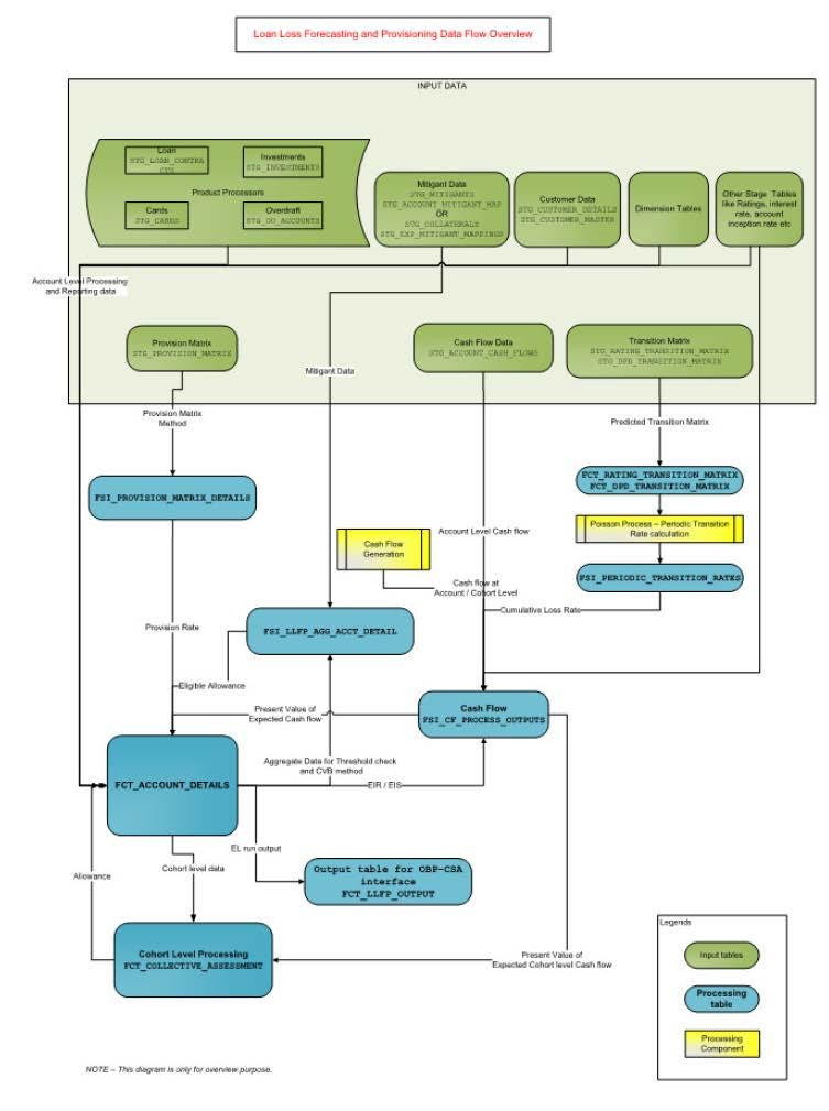
145 144