2. Explain the notion of the marginal rate of substitution and how it relates to the utilitymaximizing

Transcription

1 LEARNING OBJECTIVES 1. Explain utility maximization using the concepts of indifference curves and budget lines. 2. Explain the notion of the marginal rate of substitution and how it relates to the utilitymaximizing solution. 3. Derive a demand curve from an indifference map. Economists typically use a different set of tools than those presented in the chapter up to this point to analyze consumer choices. While somewhat more complex, the tools presented in this section give us a powerful framework for assessing consumer choices. We will begin our analysis with an algebraic and graphical presentation of the budget constraint. We will then examine a new concept that allows us to draw a map of a consumer s preferences. Then we can draw some conclusions about the choices a utilitymaximizing consumer could be expected to make. The Budget Line As we have already seen, a consumer s choices are limited by the budget available. Total spending for goods and services can fall short of the budget constraint but may not exceed it. Algebraically, we can write the budget constraint for two goods X and Y as: Equation 7.7 PXQX+PYQY B where PX and PY are the prices of goods X and Y and QX and QY are the quantities of goods X and Y chosen. The total income available to spend on the two goods is B, the consumer s budget. Equation 7.7states that total expenditures on goods X and Y (the left-hand side of the equation) cannot exceed B. 350

2 Suppose a college student, Janet Bain, enjoys skiing and horseback riding. A day spent pursuing either activity costs $50. Suppose she has $250 available to spend on these two activities each semester. Ms. Bain s budget constraint is illustrated in Figure 7.9 "The Budget Line". For a consumer who buys only two goods, the budget constraint can be shown with a budget line. Abudget line shows graphically the combinations of two goods a consumer can buy with a given budget. The budget line shows all the combinations of skiing and horseback riding Ms. Bain can purchase with her budget of $250. She could also spend less than $250, purchasing combinations that lie below and to the left of the budget line in Figure 7.9 "The Budget Line". Combinations above and to the right of the budget line are beyond the reach of her budget. Figure 7.9 The Budget Line 351

3 The budget line shows combinations of the skiing and horseback riding Janet Bain could consume if the price of each activity is $50 and she has $250 available for them each semester. The slope of this budget line is 1, the negative of the price of horseback riding divided by the price of skiing. The vertical intercept of the budget line (point D) is given by the number of days of skiing per month that Ms. Bain could enjoy, if she devoted all of her budget to skiing and none to horseback riding. She has $250, and the price of a day of skiing is $50. If she 352

4 spent the entire amount on skiing, she could ski 5 days per semester. She would be meeting her budget constraint, since: $ $50 5 = $250 The horizontal intercept of the budget line (point E) is the number of days she could spend horseback riding if she devoted her $250 entirely to that sport. She could purchase 5 days of either skiing or horseback riding per semester. Again, this is within her budget constraint, since: $ $50 0 = $250 Because the budget line is linear, we can compute its slope between any two points. Between points D and E the vertical change is 5 days of skiing; the horizontal change is 5 days of horseback riding. The slope is thus 5/5= 1. More generally, we find the slope of the budget line by finding the vertical and horizontal intercepts and then computing the slope between those two points. The vertical intercept of the budget line is found by dividing Ms. Bain s budget, B, by the price of skiing, the good on the vertical axis (PS). The horizontal intercept is found by dividing B by the price of horseback riding, the good on the horizontal axis (PH). The slope is thus: Equation 7.8 Slope= B/PSB/PH Simplifying this equation, we obtain Equation 7.9 Slope= BPS PHB= PHPS 353

5 After canceling, Equation 7.9 shows that the slope of a budget line is the negative of the price of the good on the horizontal axis divided by the price of the good on the vertical axis. Heads Up! It is easy to go awry on the issue of the slope of the budget line: It is the negative of the price of the good on the horizontal axis divided by the price of the good on the vertical axis. But does not slope equal the change in the vertical axis divided by the change in the horizontal axis? The answer, of course, is that the definition of slope has not changed. Notice that Equation 7.8 gives the vertical change divided by the horizontal change between two points. We then manipulated Equation 7.8 a bit to get to Equation 7.9 and found that slope also equaled the negative of the price of the good on the horizontal axis divided by the price of the good on the vertical axis. Price is not the variable that is shown on the two axes. The axes show the quantities of the two goods. Indifference Curves Suppose Ms. Bain spends 2 days skiing and 3 days horseback riding per semester. She will derive some level of total utility from that combination of the two activities. There are other combinations of the two activities that would yield the same level of total utility. Combinations of two goods that yield equal levels of utility are shown on an indifference curve.limiting the situation to two goods allows us to show the problem graphically. By stating the problem of utility maximization with equations, we could extend the analysis to any number of goods and services. Because all points along an indifference curve generate the same level of utility, economists say that a consumer is indifferent between them. Figure 7.10 "An Indifference Curve" shows an indifference curve for combinations of skiing and horseback riding that yield the same level of total utility. Point X marks Ms. Bain s initial combination of 2 days skiing and 3 days horseback riding per semester. 354

6 The indifference curve shows that she could obtain the same level of utility by moving to point W, skiing for 7 days and going horseback riding for 1 day. She could also get the same level of utility at point Y, skiing just 1 day and spending 5 days horseback riding. Ms. Bain is indifferent among combinations W, X, and Y. We assume that the two goods are divisible, so she is indifferent between any two points along an indifference curve. Figure 7.10 An Indifference Curve 355

7 The indifference curve A shown here gives combinations of skiing and horseback riding that produce the same level of utility. Janet Bain is thus indifferent to which point on the curve she selects. Any point below and to the left of the indifference curve would produce a lower level of utility; any point above and to the right of the indifference curve would produce a higher level of utility. Now look at point T in Figure 7.10 "An Indifference Curve". It has the same amount of skiing as point X, but fewer days are spent horseback riding. Ms. Bain would thus prefer point X to point T. Similarly, she prefers X to U. What about a choice between the combinations at point W and point T? Because combinations X and W are equally satisfactory, and because Ms. Bain prefers X to T, she must prefer W to T. In general, any combination of two goods that lies below and to the left of an indifference curve for those goods yields less utility than any combination on the indifference curve. Such combinations are inferior to combinations on the indifference curve. Point Z, with 3 days of skiing and 4 days of horseback riding, provides more of both activities than point X; Z therefore yields a higher level of utility. It is also superior to point W. In general, any combination that lies above and to the right of an indifference curve is preferred to any point on the indifference curve. We can draw an indifference curve through any combination of two goods. Figure 7.11 "Indifference Curves" shows indifference curves drawn through each of the points we have discussed. Indifference curve A from Figure 7.10 "An Indifference Curve" is inferior to indifference curve B. Ms. Bain prefers all the combinations on indifference curve B to those on curve A, and she regards each of the combinations on indifference curve C as inferior to those on curves A and B. Although only three indifference curves are shown in Figure 7.11 "Indifference Curves", in principle an infinite number could be drawn. The collection of indifference curves for a consumer constitutes a kind of map illustrating a consumer s preferences. Different 356

8 consumers will have different maps. We have good reason to expect the indifference curves for all consumers to have the same basic shape as those shown here: They slope downward, and they become less steep as we travel down and to the right along them. Figure 7.11 Indifference Curves 357

9 Each indifference curve suggests combinations among which the consumer is indifferent. Curves that are higher and to the right are preferred to those that are lower and to the left. Here, indifference curve B is preferred to curve A, which is preferred to curve C. The slope of an indifference curve shows the rate at which two goods can be exchanged without affecting the consumer s utility. Figure 7.12 "The Marginal Rate of Substitution" shows indifference curve C from Figure 7.11 "Indifference Curves". Suppose Ms. Bain is at point S, consuming 4 days of skiing and 1 day of horseback riding per semester. Suppose she spends another day horseback riding. This additional day of horseback riding does not affect her utility if she gives up 2 days of skiing, moving to point T. She is thus willing to give up 2 days of skiing for a second day of horseback riding. The curve shows, however, that she would be willing to give up at most 1 day of skiing to obtain a third day of horseback riding (shown by point U). Figure 7.12 The Marginal Rate of Substitution 358

10 The marginal rate of substitution is equal to the absolute value of the slope of an indifference curve. It is the maximum amount of one good a consumer is willing to give up to obtain an additional unit of another. Here, it is the number of days of skiing Janet Bain would be willing to give up to obtain an additional day of horseback riding. Notice that the marginal rate of substitution (MRS) declines as she consumes more and more days of horseback riding. 359

11 The maximum amount of one good a consumer would be willing to give up in order to obtain an additional unit of another is called the marginal rate of substitution (MRS), which is equal to the absolute value of the slope of the indifference curve between two points. Figure 7.12 "The Marginal Rate of Substitution" shows that as Ms. Bain devotes more and more time to horseback riding, the rate at which she is willing to give up days of skiing for additional days of horseback riding her marginal rate of substitution diminishes. The Utility-Maximizing Solution We assume that each consumer seeks the highest indifference curve possible. The budget line gives the combinations of two goods that the consumer can purchase with a given budget. Utility maximization is therefore a matter of selecting a combination of two goods that satisfies two conditions: 1. The point at which utility is maximized must be within the attainable region defined by the budget line. 2. The point at which utility is maximized must be on the highest indifference curve consistent with condition 1. Figure 7.13 "The Utility-Maximizing Solution" combines Janet Bain s budget line from Figure 7.9 "The Budget Line" with her indifference curves from Figure 7.11 "Indifference Curves". Our two conditions for utility maximization are satisfied at point X, where she skis 2 days per semester and spends 3 days horseback riding. Figure 7.13 The Utility-Maximizing Solution 360

12 Combining Janet Bain s budget line and indifference curves from Figure 7.9 "The Budget Line" and Figure 7.11 "Indifference Curves", we find a point that (1) satisfies the budget constraint and (2) is on the highest indifference curve possible. That occurs for Ms. Bain at point X. The highest indifference curve possible for a given budget line is tangent to the line; the indifference curve and budget line have the same slope at that point. The absolute value 361

13 of the slope of the indifference curve shows themrs between two goods. The absolute value of the slope of the budget line gives the price ratio between the two goods; it is the rate at which one good exchanges for another in the market. At the point of utility maximization, then, the rate at which the consumer is willing to exchange one good for another equals the rate at which the goods can be exchanged in the market. For any two goods X and Y, with good X on the horizontal axis and good Y on the vertical axis, Equation 7.10 MRSX,Y=PXPY Utility Maximization and the Marginal Decision Rule How does the achievement of The Utility Maximizing Solution in Figure 7.13 "The Utility-Maximizing Solution" correspond to the marginal decision rule? That rule says that additional units of an activity should be pursued, if the marginal benefit of the activity exceeds the marginal cost. The observation of that rule would lead a consumer to the highest indifference curve possible for a given budget. Suppose Ms. Bain has chosen a combination of skiing and horseback riding at point S in Figure 7.14 "Applying the Marginal Decision Rule". She is now on indifference curve C. She is also on her budget line; she is spending all of the budget, $250, available for the purchase of the two goods. Figure 7.14Applying the Marginal Decision Rule 362

14 Suppose Ms. Bain is initially at point S. She is spending all of her budget, but she is not maximizing utility. Because her marginal rate of substitution exceeds the rate at which the market asks her to give up skiing for horseback riding, she can increase her satisfaction by moving to point D. Now she is on a higher indifference curve, E. She will continue exchanging skiing for horseback riding until she reaches point X, at which she is on curve A, the highest indifference curve possible. 363

15 An exchange of two days of skiing for one day of horseback riding would leave her at point T, and she would be as well off as she is at point S. Her marginal rate of substitution between points S and T is 2; her indifference curve is steeper than the budget line at point S. The fact that her indifference curve is steeper than her budget line tells us that the rate at which she is willing to exchange the two goods differs from the rate the market asks. She would be willing to give up as many as 2 days of skiing to gain an extra day of horseback riding; the market demands that she give up only one. The marginal decision rule says that if an additional unit of an activity yields greater benefit than its cost, it should be pursued. If the benefit to Ms. Bain of one more day of horseback riding equals the benefit of 2 days of skiing, yet she can get it by giving up only 1 day of skiing, then the benefit of that extra day of horseback riding is clearly greater than the cost. Because the market asks that she give up less than she is willing to give up for an additional day of horseback riding, she will make the exchange. Beginning at point S, she will exchange a day of skiing for a day of horseback riding. That moves her along her budget line to point D. Recall that we can draw an indifference curve through any point; she is now on indifference curve E. It is above and to the right of indifference curve C, so Ms. Bain is clearly better off. And that should come as no surprise. When she was at point S, she was willing to give up 2 days of skiing to get an extra day of horseback riding. The market asked her to give up only one; she got her extra day of riding at a bargain! Her move along her budget line from point S to point D suggests a very important principle. If a consumer s indifference curve intersects the budget line, then it will always be possible for the consumer to make exchanges along the budget line that move to a higher indifference curve. Ms. Bain s new indifference curve at point D also intersects her budget line; she s still willing to give up more skiing than the market asks for additional riding. She will make another exchange and move along her budget line to point X, at which she attains the highest indifference curve possible with her budget. Point X is on indifference curve A, which is tangent to the budget line. 364

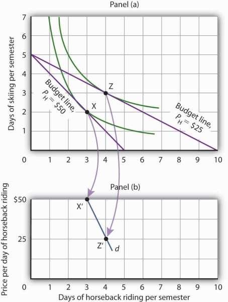
16 Having reached point X, Ms. Bain clearly would not give up still more days of skiing for additional days of riding. Beyond point X, her indifference curve is flatter than the budget line her marginal rate of substitution is less than the absolute value of the slope of the budget line. That means that the rate at which she would be willing to exchange skiing for horseback riding is less than the market asks. She cannot make herself better off than she is at point X by further rearranging her consumption. Point X, where the rate at which she is willing to exchange one good for another equals the rate the market asks, gives her the maximum utility possible. Utility Maximization and Demand Figure 7.14 "Applying the Marginal Decision Rule" showed Janet Bain s utilitymaximizing solution for skiing and horseback riding. She achieved it by selecting a point at which an indifference curve was tangent to her budget line. A change in the price of one of the goods, however, will shift her budget line. By observing what happens to the quantity of the good demanded, we can derive Ms. Bain s demand curve. Panel (a) of Figure 7.15 "Utility Maximization and Demand" shows the original solution at point X, where Ms. Bain has $250 to spend and the price of a day of either skiing or horseback riding is $50. Now suppose the price of horseback riding falls by half, to $25. That changes the horizontal intercept of the budget line; if she spends all of her money on horseback riding, she can now ride 10 days per semester. Another way to think about the new budget line is to remember that its slope is equal to the negative of the price of the good on the horizontal axis divided by the price of the good on the vertical axis. When the price of horseback riding (the good on the horizontal axis) goes down, the budget line becomes flatter. Ms. Bain picks a new utility-maximizing solution at point Z. Figure 7.15 Utility Maximization and Demand 365

17 366

18 By observing a consumer s response to a change in price, we can derive the consumer s demand curve for a good. Panel (a) shows that at a price for horseback riding of $50 per day, Janet Bain chooses to spend 3 days horseback riding per semester. Panel (b) shows that a reduction in the price to $25 increases her quantity demanded to 4 days per semester. Points X and Z, at which Ms. Bain maximizes utility at horseback riding prices of $50 and $25, respectively, become points X and Z on her demand curve, d, for horseback riding in Panel (b). The solution at Z involves an increase in the number of days Ms. Bain spends horseback riding. Notice that only the price of horseback riding has changed; all other features of the utility-maximizing solution remain the same. Ms. Bain s budget and the price of skiing are unchanged; this is reflected in the fact that the vertical intercept of the budget line remains fixed. Ms. Bain s preferences are unchanged; they are reflected by her indifference curves. Because all other factors in the solution are unchanged, we can determine two points on Ms. Bain s demand curve for horseback riding from her indifference curve diagram. At a price of $50, she maximized utility at point X, spending 3 days horseback riding per semester. When the price falls to $25, she maximizes utility at point Z, riding 4 days per semester. Those points are plotted as points X and Z on her demand curve for horseback riding in Panel (b) of Figure 7.15 "Utility Maximization and Demand". KEY TAKEAWAYS A budget line shows combinations of two goods a consumer is able to consume, given a budget constraint. An indifference curve shows combinations of two goods that yield equal satisfaction. To maximize utility, a consumer chooses a combination of two goods at which an indifference curve is tangent to the budget line. At the utility-maximizing solution, the consumer s marginal rate of substitution (the absolute value of the slope of the indifference curve) is equal to the price ratio of the two goods. 367

19 We can derive a demand curve from an indifference map by observing the quantity of the good consumed at different prices. TRY IT! 1. Suppose a consumer has a budget for fast-food items of $20 per week and spends this money on two goods, hamburgers and pizzas. Suppose hamburgers cost $5 each and pizzas cost $10. Put the quantity of hamburgers purchased per week on the horizontal axis and the quantity of pizzas purchased per week on the vertical axis. Draw the budget line. What is its slope? 2. Suppose the consumer in part (a) is indifferent among the combinations of hamburgers and pizzas shown. In the grid you used to draw the budget lines, draw an indifference curve passing through the combinations shown, and label the corresponding points A, B, and C. Label this curve I. Combination Hamburgers/week Pizzas/week A 5 0 B 3 ½ C The budget line is tangent to indifference curve I at B. Explain the meaning of this tangency. Case in Point: Preferences Prevail in P.O.W. Camps Economist R. A. Radford spent time in prisoner of war (P.O.W.) camps in Italy and Germany during World War II. He put this unpleasant experience to good use by testing a number of economic theories there. Relevant to this chapter, he consistently observed utility-maximizing behavior. In the P.O.W. camps where he stayed, prisoners received rations, provided by their captors and the Red Cross, including tinned milk, tinned beef, jam, butter, biscuits, 368

20 chocolate, tea, coffee, cigarettes, and other items. While all prisoners received approximately equal official rations (though some did manage to receive private care packages as well), their marginal rates of substitution between goods in the ration packages varied. To increase utility, prisoners began to engage in trade. Prices of goods tended to be quoted in terms of cigarettes. Some camps had better organized markets than others but, in general, even though prisoners of each nationality were housed separately, so long as they could wander from bungalow to bungalow, the cigarette prices of goods were equal across bungalows. Trade allowed the prisoners to maximize their utility. Consider coffee and tea. Panel (a) shows the indifference curves and budget line for typical British prisoners and Panel (b) shows the indifference curves and budget line for typical French prisoners. Suppose the price of an ounce of tea is 2 cigarettes and the price of an ounce of coffee is 1 cigarette. The slopes of the budget lines in each panel are identical; all prisoners faced the same prices. The price ratio is 1/2. Suppose the ration packages given to all prisoners contained the same amounts of both coffee and tea. But notice that for typical British prisoners, given indifference curves which reflect their general preference for tea, the MRS at the initial allocation (point A) is less than the price ratio. For French prisoners, the MRS is greater than the price ratio (point B). By trading, both British and French prisoners can move to higher indifference curves. For the British prisoners, the utility-maximizing solution is at point E, with more tea and little coffee. For the French prisoners the utility-maximizing solution is at point E, with more coffee and less tea. In equilibrium, both British and French prisoners consumed tea and coffee so that their MRS s equal 1/2, the price ratio in the market. Figure

21 Source: R. A. Radford, The Economic Organisation of a P.O.W. Camp, Economica 12 (November 1945): ; and Jack Hirshleifer, Price Theory and Applications (Englewood Cliffs, NJ: Prentice Hall, 1976): ANSWERS TO TRY IT! P ROBLEMS 1. The budget line is shown in Panel (a). Its slope is $5/$10 = Panel (b) shows indifference curve I. The points A, B, and C on I have been labeled. 3. The tangency point at B shows the combinations of hamburgers and pizza that maximize the consumer s utility, given the budget constraint. At the point of tangency, the marginal rate of substitution (MRS) between the two goods is equal to the ratio of prices of the two goods. This means that the rate at which the consumer is willing to exchange one good for another equals the rate at which the goods can be exchanged in the market. Figure

22 7.4 Review and Practice Summary In this chapter we have examined the model of utility-maximizing behavior. Economists assume that consumers make choices consistent with the objective of achieving the maximum total utility possible for a given budget constraint. Utility is a conceptual measure of satisfaction; it is not actually measurable. The theory of utility maximization allows us to ask how a utility-maximizing consumer would respond to a particular event. By following the marginal decision rule, consumers will achieve the utility-maximizing condition: Expenditures equal consumers budgets, and ratios of marginal utility to price are equal for all pairs of goods and services. Thus, consumption is arranged so that the extra utility per dollar spent is equal for all goods and services. The marginal utility from a particular good or service eventually diminishes as consumers consume more of it during a period of time. 371

23 Utility maximization underlies consumer demand. The amount by which the quantity demanded changes in response to a change in price consists of a substitution effect and an income effect. The substitution effect always changes quantity demanded in a manner consistent with the law of demand. The income effect of a price change reinforces the substitution effect in the case of normal goods, but it affects consumption in an opposite direction in the case of inferior goods. An alternative approach to utility maximization uses indifference curves. This approach does not rely on the concept of marginal utility, and it gives us a graphical representation of the utility-maximizing condition. CONCEPT PROBLEMS 1. Suppose you really, really like ice cream. You adore ice cream. Does the law of diminishing marginal utility apply to your ice cream consumption? 2. If two commodities that you purchase on a regular basis carry the same price, does that mean they both provide the same total utility? Marginal utility? 3. If a person goes to the bowling alley planning to spend $15 but comes away with $5, what, if anything, can you conclude about the marginal utility of the alternatives (for example, bowl another line, have a soda or a sandwich) available to the person at the time he or she leaves? 4. Which do you like more going to the movies or watching rented DVDs at home? If you engage in both activities during the same period, say a week, explain why. 5. Do you tend to eat more at a fixed-price buffet or when ordering from an a la carte menu? Explain, using the marginal decision rule that guides your behavior. 6. Suppose there is a bill to increase the tax on cigarettes by $1 per pack coupled with an income tax cut of $500. Suppose a person smokes an average of 500 packs of cigarettes per year and would thus face a tax increase of about $500 per year from the cigarette tax at the person s current level of consumption. The income tax measure would increase the person s after-tax income by $500. Would the combined measures be likely to have any effect on the person s consumption of cigarettes? Why or why not? 372

24 7. How does an increase in income affect a consumer s budget line? His or her total utility? 8. Why can Ms. Bain not consume at point Y in Figure 7.13 "The Utility-Maximizing Solution"? 9. Suppose Ms. Bain is now consuming at point V in Figure 7.13 "The Utility-Maximizing Solution". Use the marginal decision rule to explain why a shift to X would increase her utility. 10. Suppose that you are a utility maximizer and so is your economics instructor. What can you conclude about your respective marginal rates of substitution for movies and concerts? NUMERICAL PROBLEMS 1. The table shows the total utility Joseph derives from eating pizza in the evening while studying. Pieces of pizza/evening Total Utility How much marginal utility does Joseph derive from the third piece of pizza? 2. After eating how many pieces of pizza does marginal utility start to decline? 3. If the pizza were free, what is the maximum number of pieces Joseph would eat in an evening? 373

25 4. On separate diagrams, construct Joseph s total utility and marginal utility curves for pizza. Does the law of diminishing marginal utility hold? How do you know? 2. Suppose the marginal utility of good A is 20 and its price is $4, and the marginal utility of good B is 50 and its price is $5. The individual to whom this information applies is spending $20 on each good. Is he or she maximizing satisfaction? If not, what should the individual do to increase total satisfaction? On the basis of this information, can you pick an optimum combination? Why or why not? 3. John and Marie settle down to watch the evening news. Marie is content to watch the entire program, while John continually switches channels in favor of possible alternatives. Draw the likely marginal utility curves for watching the evening news for the two individuals. Whose marginal utility curve is likely to be steeper? 4. Li, a very careful maximizer of utility, consumes two services, going to the movies and bowling. She has arranged her consumption of the two activities so that the marginal utility of going to a movie is 20 and the marginal utility of going bowling is 10. The price of going to a movie is $10, and the price of going bowling is $5. Show that she is satisfying the requirement for utility maximization. Now show what happens when the price of going bowling rises to $ The table shows the total utility (TU) that Jeremy receives from consuming different amounts of two goods, X and Y, per month. Quantity TU X MU X MU X /P X TU Y MU Y MU Y /P Y

26 Quantity TU X MU X MU X /P X TU Y MU Y MU Y /P Y Fill in the other columns of the table by calculating the marginal utilities for goods X and Y and the ratios of marginal utilities to price for the two goods. Assume that the price of both goods X and Y is $3. Be sure to use the midpoint convention when you fill out the table. 2. If Jeremy allocates $30 to spend on both goods, how many units will he buy of each? 3. How much will Jeremy spend on each good at the utility maximizing combination? 4. How much total utility will Jeremy experience by buying the utility-maximizing combination? 5. Suppose the price of good Y increases to $6. How many units of X and Y will he buy to maximize his utility now? 6. Draw Jeremy s demand curve for good Y between the prices of $6 and $3. 6. Sid is a commuter-student at his college. During the day, he snacks on cartons of yogurt and the house special sandwiches at the Student Center cafeteria. A carton of yogurt costs $1.20; the Student Center often offers specials on the sandwiches, so their price varies a great deal. Sid has a budget of $36 per week for food at the Center. Five of Sid s indifference curves are given by the schedule below; the points listed in the tables correspond to the points shown in the graph. Figure

27 1. Use the set of Sid s indifference curves shown as a guide in drawing your own graph grid. Draw Sid s indifference curves and budget line, assuming sandwiches cost $3.60. Identify the point at which he maximizes utility. How many sandwiches will he consume? How many cartons of yogurt? (Hint: All of the answers in this exercise occur at one of the combinations given in the tables on this page.) 376

28 2. Now suppose the price of sandwiches is cut to $1.20. Draw the new budget line. Identify the point at which Sid maximizes utility. How many sandwiches will he consume? How many cartons of yogurt? 3. Now draw the budget lines implied by a price of yogurt of $1.20 and sandwich prices of $0.90 and $1.80. With the observations you ve already made for sandwich prices of $3.60 and $1.20, draw the demand curve. Explain how this demand curve illustrates the law of demand. 7. Consider a consumer who each week purchases two goods, X and Y. The following table shows three different combinations of the two goods that lie on three of her indifference curves A,B, and C. Indifference Curve Quantities of goods X and Y, respectively Quantitities of goods X and Y, respectively Quantities of goods X and Y, respectively A 1 unit of X and 4 of Y 2 units of X and 2 of Y 3 units of X and 1 of Y B 1 unit of X and 7 of Y 3 units of X and 2 of Y 5 units of X and 1 of Y C 2 units of X and 5 of Y 4 units of X and 3 of Y 7 units of X and 2 of Y 1. With good X on the horizontal axis and good Y on the vertical axis, draw the implied indifference curves. Be sure to label all curves and axes completely. 2. On Curve A, what is the marginal rate of substitution (MRS) between the first two combinations of goods X and Y? 3. Suppose this consumer has $500 available to spend on goods X and Y and that each costs $100. Add her budget line to the graph you drew in part (a). What is the slope of the budget line? 4. What is the utility-maximizing combination of goods X and Y for this consumer? (Assume in this exercise that the utility-maximizing combination always occurs at one of the combinations shown in the table.) 5. What is the MRS at the utility-maximizing combination? 377

29 6. Now suppose the price of good X falls to $50. Draw the new budget line onto your graph and identify the utility-maximizing combination. What is the MRS at the utilitymaximizing combination? How much of each good does she consume? 7. Draw the demand curve for good X between prices of $50 and $100, assuming it is linear in this range. 378

30 Chapter 8 Production and Cost Start Up: Street Cleaning Around the World It is dawn in Shanghai, China. Already thousands of Chinese are out cleaning the city s streets. They are using brooms. On the other side of the world, night falls in Washington, D.C., where the streets are also being cleaned by a handful of giant street-sweeping machines driven by a handful of workers. The difference in method is not the result of a greater knowledge of modern technology in the United States the Chinese know perfectly well how to build street-sweeping machines. It is a production decision based on costs in the two countries. In China, where wages are relatively low, an army of workers armed with brooms is the least expensive way to produce clean streets. In Washington, where labor costs are high, it makes sense to use more machinery and less labor. All types of production efforts require choices in the use of factors of production. In this chapter we examine such choices. Should a good or service be produced using relatively more labor and less capital? Or should relatively more capital and less labor be used? What about the use of natural resources? In this chapter we see why firms make the production choices they do and how their costs affect their choices. We will apply the marginal decision rule to the production process and see how this rule ensures that production is carried out at the lowest cost possible. We examine the nature of production and costs in order to gain a better understanding of supply. We thus shift our focus to firms, organizations that produce 379